# Sustainability in Supply Chain Management {#sec-nachhaltigkeit}
```{r ch9-setup}
#| include: false
library(dplyr)
library(tidyr)
library(readr)
library(ggplot2)
library(knitr)
library(kableExtra)
# Load functions and colour palette from scm_functions.R (object `cols`)
source("../R/scm_functions.R")
```
::: {.lernziele}
**Learning objectives**
- Classify sustainability in supply chain management using the Brundtland definition and the triple bottom line (economic, environmental, social)
- Explain the relationship between sustainability goals and the tetrahedron of trade-offs from Chapter [-@sec-logistikkosten] and give your own trade-off examples
- Position companies in the strategic fit grid according to environmental exposure and environmental orientation
- Distinguish the hierarchy of environmental SCM strategies – rules of action, basic strategies (sufficiency, efficiency, consistency), basic principles and concepts – and link them to practical examples
- Explain the waste hierarchy and the concept of the circular economy, and differentiate between linear, reverse and circular supply chains
- Name the design fields circular product design, sustainable logistics and circular production and assign examples to them
- Import emissions data in R with `readr`, normalise it into an index with `dplyr` and visualise it comparatively as a stacked bar chart with `ggplot2::geom_col()`
- Apply the generic strategies of the circular supply chain (product complexity × dynamics of customer preferences) to specific products
:::
## A fifth dimension of the system of objectives
In Chapter [-@sec-logistikkosten] we depicted the logistics system of objectives as a **tetrahedron**: quality, speed, cost and flexibility/resilience form four vertices between which every logistics system has to position itself, because an improvement at one vertex almost always comes at the expense of at least one other. This view was deliberately limited to the *classic* performance dimensions of logistics – that is, the variables by which supply chains have primarily been measured for decades.
For some years now, this system of objectives has been joined by a further, independent dimension that cannot be fitted seamlessly into any of the four vertices of the tetrahedron and is therefore treated separately in this chapter: **sustainability**. Sustainability is not a "fifth vertex" that simply sits alongside the other four, but a cross-cutting dimension that affects *each* of the four original vertices – cost (e.g. through carbon pricing or investment in low-emission vehicles), speed (e.g. when a lower-emission rail connection takes longer than the lorry), quality (e.g. through requirements for recycled materials) and flexibility (e.g. when take-back systems tie up additional capacity). Anyone who takes sustainability in supply chain management seriously must therefore follow the same trade-off logic we have already encountered for the classic tetrahedron – except that an additional objective, often difficult to monetise, now enters the trade-off.
This chapter addresses this dimension. It deepens the sustainability content of the lecture unit "Objectives, trade-offs and logistics costs" and therefore follows directly on from Chapter [-@sec-logistikkosten]. We first clarify what sustainability actually means in the SCM context, then examine how companies can respond strategically to environmental requirements, systematise the multitude of environmental SCM strategies in a hierarchy, turn to the circular economy as a central design principle and finally use our own R calculation to investigate how the central trade-off between sustainability and the classic logistics objectives can be quantified using a concrete example – the choice of transport mode.
## What does sustainability mean in supply chain management?
The term "sustainability" is used so inflationarily today that a clear definition is essential before we apply it to supply chains. The most influential definition to this day comes from the United Nations' Brundtland Report, published in 1987:
::: {.definition}
**Definition: Sustainability**
A social system is described as **sustainable** if it can be regarded as both intragenerationally and intergenerationally just. Just means that it "meets the needs of the present without compromising the ability of future generations to meet their own needs" [@hauff1987zukunft].
:::
Two aspects of this definition deserve particular attention. First, it refers to **intragenerational** justice – that is, justice *within* the generation living today, for instance between industrialised and developing countries or between different population groups. Second, it refers to **intergenerational** justice – justice *between* present and future generations. From the outset, sustainability is therefore not a purely environmental concept but explicitly a social and economic one as well: resources must not be consumed today in such a way that future generations can no longer meet their own needs, and this constraint applies equally to natural, social and economic "resources".
From this combination of economic, environmental and social aspects emerged the most widespread classification scheme in sustainability management: the **triple bottom line** [@baumast2013nachhaltigkeitsmanagement]. It distinguishes three equally ranked target dimensions whose joint fulfilment – not the one-sided maximisation of a single dimension – is regarded as sustainable:
- the **economic dimension**: lasting competitiveness, profitability and value creation – ultimately the classic objectives that we have already discussed in detail in Chapter [-@sec-logistikkosten],
- the **environmental dimension**: conserving natural resources, avoiding and reducing emissions and maintaining the functioning of ecosystems,
- the **social dimension**: decent working conditions along the entire supply chain, health protection, equal opportunities and social participation.
From this, a workable working definition for supply chain management can be derived, which guides this chapter:
::: {.definition}
**Definition: Sustainable supply chain management**
**Sustainable supply chain management (sustainable SCM)** refers to the planning, execution and control of business processes taking into account economic, environmental and social objectives in order to ensure the long-term competitiveness of the supply chain [@bouchery2016sustainable].
:::
What is remarkable about this definition is that it does **not** frame sustainability as the opposite of competitiveness, but as its prerequisite: a supply chain that ignores its environmental and social impacts risks reputational damage, regulatory intervention, rising raw material prices and the loss of market access – and thus ultimately precisely the economic competitiveness it actually wanted to protect by neglecting sustainability. Sustainability and classic SCM objectives therefore stand in a dual relationship: in the short term often in conflict (more sustainability usually costs money or time at first), but complementary in the long term (a lack of sustainability jeopardises competitiveness itself).
## The environmental strategic fit: how companies respond to environmental requirements
Not every company is affected by environmental issues to the same extent, and not every company responds equally offensively to a given level of exposure. To systematise this observation, a two-dimensional grid can be constructed – analogous to the strategic fit concept from Chapter [-@sec-strategic-fit] [@guenther2008oekologieorientiertes]:
- the company's **environmental exposure** (low to high): How strongly does business success depend on natural resources, emission regulations or environmental reputational risks?
- the company's **environmental orientation** (low to high): How actively does the company position itself strategically on environmental issues?
Combining the two dimensions yields four ideal-typical positions, summarised in the following table:
```{r ch9-strategic-fit}
tibble(
  Typ = c("Environmental ignorance", "Environmental resistance", "Environmental adaptation", "Environmental offensive"),
  Betroffenheit = c("low", "high", "high", "low"),
  Ökologieorientierung = c("low", "low", "high", "high"),
  Reaktionsmuster = c(
    "Environmental issues are treated as strategically secondary.",
    "Only minimum regulatory adjustment; investments are delayed, sometimes lobbying against stricter requirements.",
    "Active adaptation to environmental requirements to secure resilience and competitiveness.",
    "Sustainability is actively used as an opportunity for innovation and competitive advantage."
  ),
  Beispiele = c(
    "Volkswagen (diesel scandal, delayed EV strategy)",
    "SKW Piesteritz (chemical industry)",
    "EON (expansion of renewable generation); Stegra (green steel)",
    "Patagonia (repair service, circular approaches); IKEA (renewable energy, sustainable materials)"
  )
) |>
  kable(align = "lllll",
        col.names = c("Type", "Exposure", "Environmental orientation", "Response pattern", "Examples"),
        caption = "Four positions in the grid of environmental exposure and environmental orientation") |>
  kable_styling(font_size = 12)
```
The axes are to be read such that the upper half of the grid (high exposure) comprises companies that can hardly escape environmental requirements – they respond either defensively (resistance) or adaptively (adaptation). In the lower half (low exposure), by contrast, there is a choice: environmental issues can be ignored or used offensively as a differentiating feature, even though there is no immediate pressure. The four positions thus show that exposure alone does not determine a strategy: SKW Piesteritz and EON are both highly exposed to environmental issues because of their industry, but respond to them very differently – the one in a minimalist, wait-and-see manner (environmental resistance), the other by actively transforming its own business model (environmental adaptation). This has an important consequence for supply chain management: a company's own position in the grid directly influences which of the strategies presented below are seriously considered at all – an environmentally offensive company will be more willing to invest in circular product design or remanufacturing than an environmentally resistant one.
## From rules of action to concepts: a hierarchy of environmental SCM strategies
In practice there is an almost unmanageable variety of individual measures with which companies respond to environmental requirements – from route optimisation and recycling rates to car sharing. To provide orientation within this variety, a **four-level hierarchy model** of environmentally oriented business can be constructed, ranging from very general rules of action to concrete concepts that can be implemented directly [@dyckhoff2008nachhaltige]. The logic of this hierarchy is deductive: rules of action justify basic strategies, basic strategies are operationalised through basic principles, and basic principles finally lead to concrete concepts that can actually be implemented in individual companies.
At the top level are four **rules of action**, which formulate the conditions under which economic activity can be regarded as environmentally sustainable: keeping ecological systems healthy (e.g. IKEA's certified timber sourcing), respecting the absorptive capacity of ecological systems (e.g. emissions monitoring in chemical parks based on pollution limits), balanced use of renewable resources (e.g. fishing quotas based on the reproductive capacity of stocks) and balanced use of non-renewable resources (e.g. aluminium recycling to conserve primary raw materials). These four rules translate the abstract Brundtland definition into concrete requirements for dealing with natural systems.
From these rules of action, three **basic strategies** can be derived, often also referred to as the "three big S" of environmental strategy: **sufficiency** aims at lower absolute resource consumption through less, slower or more needs-based consumption – for instance when Patagonia deliberately promotes repairs instead of new purchases, or when sharing models encourage the collective rather than individual use of products. **Efficiency** means achieving the same or a higher output with less energy and material input – for instance through route optimisation in logistics or the conversion of store networks to LED lighting, which requires significantly less electricity for the same lighting output. **Consistency**, finally, seeks to design material and energy flows to be compatible with nature from the outset, for instance through closed material loops (Interface for carpet tiles) or the replacement of fossil energy sources with renewable ones. The difference between these three strategies is important: sufficiency reduces consumption in absolute terms, efficiency reduces it relative to the output delivered, and consistency changes the type of material and energy flows used without necessarily reducing their quantity.
At the third level are four **basic principles**, which describe *how* companies implement the basic strategies organisationally. The **responsibility principle** requires those who cause environmental impacts to also take responsibility for their consequences – for instance within the framework of extended producer responsibility for packaging or systematic carbon accounting that attributes emissions to a company's own value creation. The **cooperation principle** assumes that environmental problems can be solved better through collaboration than through isolated individual action, for instance in the form of industry initiatives for sustainable supply chains or industrial symbiosis, in which the waste heat or by-products of one plant are used by another. The **circularity principle** calls for materials to be kept in circulation for as long as possible – a principle to which we devote the next section in detail. And the **principle of function orientation** places the desired function rather than the physical product at the centre: car sharing sells mobility instead of vehicle ownership, "light as a service" sells lighting instead of a stock of lamps.
Finally, at the lowest and most concrete level are four **concepts** with which companies implement the basic principles in day-to-day business: **dematerialisation** replaces material processes with digital solutions (digital instead of printed invoices, streaming instead of physical media); **increasing energy efficiency** delivers the same output with less energy input (heat recovery in production); **decoupling** breaks problematic links between economic growth and resource consumption (working from home instead of commuting, regional instead of global sourcing); and **deceleration** relies on slower, longer-lasting usage patterns (slow fashion instead of short collection cycles, rail instead of air for business travel). The following table summarises this four-level hierarchy with one practical example each.
```{r ch9-strategien-tabelle}
tibble(
  Ebene = c(
    rep("Rule of action", 4),
    rep("Basic strategy", 3),
    rep("Basic principle", 4),
    rep("Concept", 4)
  ),
  Bezeichnung = c(
    "Keeping ecological systems healthy",
    "Respecting absorptive capacity",
    "Use of renewable resources",
    "Use of non-renewable resources",
    "Sufficiency", "Efficiency", "Consistency",
    "Responsibility principle", "Cooperation principle",
    "Circularity principle", "Function orientation",
    "Dematerialisation", "Increasing energy efficiency",
    "Decoupling", "Deceleration"
  ),
  Beispiel = c(
    "IKEA: certified/recycled timber sourcing",
    "Chemical park with continuous emissions monitoring",
    "Fishing quotas",
    "Aluminium recycling in the packaging industry",
    "Patagonia: repair service instead of new purchase",
    "DHL: route optimisation",
    "Interface: circular carpet tiles",
    "Extended producer responsibility for packaging",
    "Industry initiatives for sustainable supply chains",
    "Renault: remanufacturing of car parts",
    "Car sharing instead of vehicle ownership",
    "Digital instead of printed invoices",
    "Heat recovery in production",
    "Working from home instead of commuting",
    "Rail instead of air for business travel"
  )
) |>
  select(-Ebene) |>
  kable(align = "ll",
        col.names = c("Name", "Example"),
        caption = "Four-level hierarchy of environmental SCM strategies: from rule of action to concept") |>
  kable_styling(font_size = 12) |>
  pack_rows("Rules of action", 1, 4) |>
  pack_rows("Basic strategies", 5, 7) |>
  pack_rows("Basic principles", 8, 11) |>
  pack_rows("Concepts", 12, 15)
```
## Planning tasks in sustainable supply chain management
Sustainability changes not only the objectives but also the **planning tasks** along the supply chain. @stindt2017 classifies these – analogous to the supply chain planning matrix from Chapter [-@sec-standort-1] – by planning level and process. At the **strategic** level, the focus is on designing a network that can accommodate return flows (take-back, reprocessing, recycling) in addition to forward flows, on selecting suppliers according to environmental and social criteria and on designing products for circularity. At the **tactical** level, capacities for return and reprocessing are dimensioned, transport modes are chosen with emissions in mind and emission budgets are allocated to sites and periods. Finally, at the **operational** level, the focus is on low-emission route planning, the control of returns and the avoidance of spoilage and waste in day-to-day business.
Stindt's central thesis is that sustainability cannot be "bolted on" as an additional, downstream planning module but must be **integrated** into existing planning tasks: each of the models covered in this course reader – facility location planning, the transportation problem, inventory planning – can be extended with environmental objectives or constraints, as already indicated in Chapter [-@sec-logistikkosten] with CO₂ prices and emission budgets.
## From the linear to the circular supply chain
Of the four basic principles in the previous section, the **circularity principle** deserves closer examination because it changes the structure of entire supply chains – not just individual processes within an unchanged chain logic. To understand this structural change, it is worth first looking at the **waste hierarchy** of the Ellen MacArthur Foundation, which ranks the fundamentally available ways of dealing with materials and products at the end of their life cycle according to environmental preferability:
```{r ch9-abfallhierarchie}
tibble(
  Rang = 1:6,
  Stufe = c("Prevent", "Reduce", "Reuse", "Recycling", "Energy Recovery", "Disposal"),
  Bedeutung = c(
    "Avoid the generation of waste in the first place (e.g. through sufficiency or function orientation)",
    "Reduce the amount of material used (efficiency)",
    "Continue to use products or components without further processing",
    "Reprocess material and use it again as a raw material",
    "Use material that can no longer be recovered for energy (e.g. incineration with heat recovery)",
    "Final disposal with as few pollutants as possible (last option)"
  )
) |>
  kable(align = "cll",
        col.names = c("Rank", "Level", "Meaning"),
        caption = "Waste hierarchy: from prevention (highest priority) to disposal (lowest priority)")
```
The hierarchy is deliberately to be read as a ranking: the higher up an option is, the more the economic and environmental value of a material is preserved, and the lower the additional resource and energy input required to use it again. **Recycling** deliberately comes only fourth: in public debate recycling is often equated with sustainability, but from an environmental point of view it is in fact only the third-best available option, because recycling itself also requires energy and processes, and part of the value added originally embodied in the product is lost.
It is precisely this ranking that underlies the concept of the **circular economy**: instead of disposing of materials after a single use, they are to be kept in the economic cycle for as long as possible at the highest possible level of the hierarchy. For supply chain design, three fundamentally different chain types can be distinguished [@dyckhoff1998grundzuege; @chopra2025supply]:
::: {.definition}
**Definition: linear, reverse and circular supply chain**
A **linear supply chain** follows the classic flow of raw material extraction → production → distribution → use → disposal, without materials flowing back into the chain after the use phase.
A **reverse supply chain** (reverse logistics) supplements this linear flow with a return flow of products, components or packaging from the end customer back to upstream stages – for instance for repair, recycling or proper disposal.
A **circular supply chain** goes one step further: it is designed from the outset so that returned materials and products are fed back fully into the production and usage cycle, so that primary resources are replaced as completely as possible by secondary resources circulating in the system.
:::
The difference between reverse and circular supply chains is more than semantic: reverse logistics can be motivated purely defensively (legal take-back obligations, warranty processing), whereas a circular supply chain anticipates the return in product and process design and thus makes higher levels of the waste hierarchy – reuse and remanufacturing rather than mere recycling – achievable from the outset.
## Design fields of sustainable and circular supply chain management
To actually implement the circular economy along a supply chain, several design fields must be addressed simultaneously, which can be roughly assigned to three areas:
- **Circular product design**: circularity is already decided during product development – through design decisions that enable later **recyclability** (e.g. single-material rather than bonded composites), through design for **reuse** (e.g. modular construction that allows individual components to be replaced instead of the whole product) and through the targeted use of **recycled content**, i.e. already recovered material as the input for new products.
- **Sustainable logistics**: physical distribution itself is optimised environmentally – through **weight reduction** of products and packaging (less weight means less energy input per transport), through **distance reduction** (regional instead of global sourcing and distribution networks) and through **transport avoidance** in the narrower sense (consolidation of shipments, higher utilisation, substitution of physical by digital processes).
- **Circular production**: production itself is also designed for circularity – through the use of **renewable energy**, through the **use of production waste** as input for other processes (industrial symbiosis) and through the **recirculation of operating and auxiliary materials** (e.g. cooling or process water), which are not disposed of after a single use but reprocessed and reused.
The middle of these three areas – sustainable logistics – directly concerns a decision already familiar to us from earlier chapters: the **choice of transport mode**. In the following section we work out with our own R calculation how strongly this choice affects the carbon footprint of a shipment.
## Sustainable choice of transport mode: a calculation exercise in R
Different modes of transport – truck, rail, inland waterway vessel, ocean vessel, aircraft – differ massively in their carbon efficiency per quantity of goods transported. The customary reference unit for this is the **tonne-kilometre** (tkm): the carriage of one tonne of cargo over a distance of one kilometre. The CO2 emissions of a specific shipment can then be approximated as
$$
E \;=\; d \cdot m \cdot f
$$
where $d$ denotes the distance travelled in kilometres, $m$ the mass transported in tonnes and $f$ the **emission factor** of the respective transport mode in grams of CO2 per tonne-kilometre (g CO2/tkm). We work with exactly this formula in the following three R asides, which at the same time introduce three R techniques not yet covered in the previous chapters: importing tabular data with `readr`, constructing an index with `dplyr` and building a stacked bar chart with `ggplot2::geom_col()`.
::: {.r-exkurs}
**R aside: importing emissions data with `readr`**
So far in this book we have almost always created data directly as a vector or `tibble` in the R code. In practice, however, data – such as emission factors from an environmental database – are usually available as a **text file**, typically in CSV format (*comma-separated values*). The `tidyverse` package `readr` provides the function `read_csv()` for this purpose, which reads a CSV file (or, as here for demonstration purposes, a CSV-formatted text) and automatically detects sensible column types – numbers are imported as `double`, text as `character`, without having to specify this by hand.
So that `read_csv()` interprets a character string as **data content** rather than as a **file path**, it is marked with the base R function `I()` ("as is"):
```{r ch9-emission-import}
# CO2 emission factors of selected transport modes in g CO2 per tonne-kilometre.
# These are rounded guide values of a realistic order of magnitude
# from the relevant transport and logistics literature, used
# here for illustrative purposes.
emissionsdaten_text <- "Verkehrstraeger,Emissionsfaktor_g_tkm,Kategorie
Truck,62,Road
Rail,22,Rail
Inland vessel,31,Water
Ocean vessel,8,Water
Aircraft,602,Air"

# read_csv() reads the (literal) text and automatically detects
# that the second column is numeric -- I() prevents the
# string from being wrongly interpreted as a file path
emissionsfaktoren <- read_csv(I(emissionsdaten_text), show_col_types = FALSE)

emissionsfaktoren |>
  arrange(Emissionsfaktor_g_tkm) |>
  kable(col.names = c("Transport mode", "g CO₂ / tkm", "Category"),
        align = "lrl",
        caption = "CO2 emission factors of selected transport modes (guide values)")
```
Even this sorted table reveals the central trade-off of a sustainable choice of transport mode: the **ocean vessel** has by far the lowest emissions per tonne-kilometre, followed by rail and inland vessel; the **truck** is considerably higher, and the **aircraft** causes almost ten times the emissions of a truck per tonne-kilometre. At the same time, it is precisely the lower-emission modes – ship and rail – that are typically slower and less flexible than the truck. This is exactly where the effect of the sustainability dimension on the classic tetrahedron vertices of speed and flexibility, described at the beginning, becomes apparent.
:::
::: {.r-exkurs}
**R aside: normalisation and index construction**
Absolute emission factors are difficult to assess intuitively ("Is 31 g CO2/tkm a lot or a little?"). In practice, indicators are therefore often **normalised**, i.e. converted to a common reference value – here to the most economical transport mode available, which receives the index base value of 100. With `dplyr::mutate()` such an index can be calculated in a single line of code, because `min()` inside `mutate()` is automatically computed over the entire column and then applied element-wise to each row:
```{r ch9-emissionsindex}
# Emission index: emission factor of each transport mode relative
# to the most economical transport mode (which receives the index value 100) --
# min() is computed once over the whole column and then used in each
# row for the division
emissionsfaktoren <- emissionsfaktoren |>
  mutate(Emissionsindex = round(Emissionsfaktor_g_tkm / min(Emissionsfaktor_g_tkm) * 100, 0))

emissionsfaktoren |>
  arrange(Emissionsindex) |>
  kable(col.names = c("Transport mode", "g CO₂ / tkm", "Category", "Index (ocean vessel = 100)"),
        align = "lrlr",
        caption = "Emission index of transport modes relative to the ocean vessel")
```
The index is immediately more intuitive than the raw values: according to it, the truck emits almost eight times and the aircraft around 75 times as much CO2 per tonne-kilometre as the ocean vessel. The same normalisation logic – a value is divided by a reference value and multiplied by 100 – is encountered regularly in practice, for instance in price indices, business cycle indicators or indeed sustainability indicators such as CO2 intensity per unit of revenue.
:::
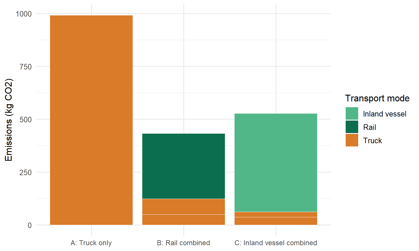
However, the pure emission factors do not yet say anything about a *specific* shipment, because a real transport chain usually combines several modes of transport. Let us consider a shipment of 20 tonnes of cargo that has to be transported over a total of around 800 kilometres and compare three scenarios: (A) truck transport throughout, (B) rail transport with pre- and on-carriage by truck to and from the terminals, and (C) inland waterway transport, also with pre- and on-carriage by truck.
```{r ch9-szenarien}
ladung_t <- 20 # tonnes of cargo per shipment, identical in all scenarios

szenarien <- tibble(
  Szenario = c(
    "A: Truck only",
    "B: Rail combined", "B: Rail combined", "B: Rail combined",
    "C: Inland vessel combined", "C: Inland vessel combined", "C: Inland vessel combined"
  ),
  Streckenabschnitt = c(
    "Main carriage",
    "Pre-carriage", "Main carriage", "On-carriage",
    "Pre-carriage", "Main carriage", "On-carriage"
  ),
  Verkehrstraeger = c(
    "Truck",
    "Truck", "Rail", "Truck",
    "Truck", "Inland vessel", "Truck"
  ),
  Distanz_km = c(800, 40, 700, 60, 30, 750, 20)
)

# Add emission factors per transport mode via left_join and
# calculate emissions per route section (g -> kg via /1000)
szenarien <- szenarien |>
  left_join(emissionsfaktoren, by = "Verkehrstraeger") |>
  mutate(Emission_kg = Distanz_km * ladung_t * Emissionsfaktor_g_tkm / 1000)

szenarien |>
  select(Szenario, Streckenabschnitt, Verkehrstraeger, Distanz_km, Emission_kg) |>
  kable(digits = 1, align = "llrrr",
        col.names = c("Scenario", "Route section", "Transport mode", "Distance (km)", "Emissions (kg)"),
        caption = "Emissions per route section and scenario (cargo: 20 t)")
```
::: {.r-exkurs}
**R aside: a stacked bar chart with `geom_col()`**
To compare the three scenarios not only in a table but also graphically, a **stacked bar chart** is a good choice: one bar per scenario, whose segments show the emissions of the individual route sections. In `ggplot2`, `geom_col()` – unlike `geom_bar()`, which *counts* frequencies – creates bars from existing `y` values; the argument `fill =` assigns each route section its own fill colour, and `ggplot2` automatically stacks the segments on top of each other as soon as several rows share the same `x` value:
```{r ch9-stacked-bar}
#| fig-cap: "CO2 emissions of three transport scenarios for a 20-tonne shipment over around 800 km"
#| fig-width: 7.5
#| fig-height: 4.5
szenarien |>
  ggplot(aes(x = Szenario, y = Emission_kg, fill = Verkehrstraeger)) +
  geom_col(color = "white", linewidth = 0.3) +
  scale_fill_manual(values = c(
    "Truck"         = cols$atp,
    "Rail"          = cols$top,
    "Inland vessel" = cols$mid
  )) +
  labs(x = NULL, y = "Emissions (kg CO2)", fill = "Transport mode") +
  theme_minimal(base_size = 12) +
  theme(axis.text.x = element_text(size = 9))
```
The stacking reveals two things at a glance: first, how much the **total height** of the bars varies between the scenarios, and second, what **share** of this total the individual route sections account for – in scenario B, for example, the rail main carriage dominates the emissions, while the truck pre- and on-carriage contribute only small segments.
:::
The calculation impressively confirms what the emission index already suggested: scenario A (truck only) causes around 992 kg CO2, scenario C (inland vessel combined) around 527 kg, and scenario B (rail combined), at around 432 kg CO2, only about 44% of the emissions of scenario A – even though the same quantity is transported over the same total distance in all three scenarios. Combined transport therefore saves a considerable amount of CO2 through the choice of main-carriage mode alone. However, this saving does not come free of charge: transhipment between truck and rail or inland vessel at the terminals costs time and money, transit time increases and flexibility decreases, because rail and ship connections run less frequently and on less flexible schedules than the truck. It is precisely this trade-off between sustainability on the one hand and speed, flexibility and sometimes also cost on the other that we place explicitly once more within the framework of the tetrahedron from Chapter [-@sec-logistikkosten] in the last substantive section of this chapter.
## Generic strategies of the circular supply chain
Circular product design cannot be pursued according to the same pattern for every product – a smartphone requires a different circular strategy than packaging. To determine the appropriate generic strategy, a two-dimensional grid of **product complexity** (low to high) and **dynamics of customer preferences** (static to dynamic) can be constructed. Combining the two dimensions yields four generic strategies:
```{r ch9-normstrategien}
tibble(
  Quadrant = c(
    "low complexity / dynamic preferences",
    "high complexity / dynamic preferences",
    "low complexity / static preferences",
    "high complexity / static preferences"
  ),
  Normstrategie = c(
    "Design for Recycling",
    "Design for Remanufacture & Reuse",
    "Design for Recycled Content",
    "Design for Repair & Durability"
  ),
  Begründung = c(
    "Short-lived, trend-dependent products are hardly worth remanufacturing; separating materials by type for material recycling is the most efficient circular option.",
    "High material value and high manufacturing complexity justify the more elaborate remanufacturing of entire components or devices, despite changing customer wishes.",
    "Simple, standardised products with stable demand are well suited to using a high proportion of recycled material already in the manufacturing process.",
    "For complex products with long-lasting demand, a design geared to repairability and a long service life pays off particularly well."
  ),
  Beispielprodukte = c(
    "Clothing, furniture",
    "Smartphones, computers",
    "Packaging, steel",
    "Cars, household appliances"
  )
) |>
  kable(align = "llll",
        col.names = c("Quadrant", "Generic strategy", "Rationale", "Example products"),
        caption = "Generic strategies of the circular supply chain by product complexity and preference dynamics") |>
  kable_styling(font_size = 12)
```
The table makes clear that the "circular economy" is not a uniform recipe but sets very different priorities depending on the product category. For packaging and steel – low complexity, stable demand – the focus is on increasing the share of recycled content, because standardised, plannable material loops can be established for this. For smartphones and computers, on the other hand, where both material value and manufacturing complexity are high, remanufacturing – the reprocessing of entire assemblies or devices for resale – pays off, even though customer preferences (new functions, new design) change constantly. Finally, for cars and household appliances, which are complex but in comparatively stable demand, a design geared to repairability from the outset pays off – a principle that links directly to the Renault example from the strategy hierarchy above.
## Case study: sustainability at SushiFresh
::: {.fallstudie}
**Case study: environmental trade-offs at SushiFresh GmbH**
SushiFresh GmbH, introduced in Chapter [-@sec-logistikkosten], provides an illustrative example of the sustainability issues faced by a fresh food producer. Three fields of action are at the forefront:
- **Food waste:** Every box left unsold in the evening is not only an economic loss (overage cost $c^o$ in the newsvendor model, Chapter [-@sec-newsvendor]) but also an environmental one: fishing resources, cooling energy and transport effort are destroyed together with the fish. Anyone who puts a monetary value on the environmental impact of unsold goods effectively increases $c^o$ – the critical ratio falls, and the optimal production quantity decreases. Here, sustainability thus directly shifts an operational decision. According to the waste hierarchy, leftover goods should also be recovered as high up as possible (evening discount before donation before disposal).
- **Cold chain and transport:** The daily, refrigerated delivery in small quantities is emissions-intensive. The location decision (Chapters [-@sec-standort-1] and [-@sec-standort-2]) influences the kilometres driven; consolidation in a central kitchen reduces inventory and spoilage (Chapter [-@sec-unsicherheit-pooling]) but tends to lengthen the distances. This reveals the trade-off between the concepts of *efficiency* (consolidation) and *decoupling* (regional, short distances).
- **Sourcing of fish:** Salmon and tuna are renewable resources, but at risk of overexploitation. The rule of action of balanced use of renewable resources (fishing quotas, certified fisheries) thus becomes a criterion for supplier selection – an example of the cooperation principle with the wholesaler Nord-Fisch (Chapter [-@sec-bullwhip]).
In the grid of exposure and environmental orientation, SushiFresh, as a food producer with perishable goods and a critical raw material, is highly exposed. Positioning itself as *environmental adaptation* – for instance through consistent waste avoidance, certified fish and reusable packaging – also fits the company's quality and freshness positioning.
:::
## Trade-offs between sustainability and classic logistics objectives
This brings us full circle back to the tetrahedron from Chapter [-@sec-logistikkosten]. The transport mode calculation in the previous section showed by way of example that sustainability objectives can rarely be pursued in isolation, but are almost always in tension with at least one of the four classic vertices of the tetrahedron:
- **Sustainability versus speed**: lower-emission combined transport (rail, inland vessel) is as a rule slower than pure truck transport, because transhipment operations and lower service frequencies cost additional time.
- **Sustainability versus flexibility/resilience**: circular supply chains require functioning reverse logistics, additional capacity for take-back, sorting and reprocessing, and stable partnerships with waste management companies and recyclers – all of which reduces the ability to respond flexibly to changes in demand in the short term.
- **Sustainability versus cost**: recycled materials, renewable energy or more elaborate, repair-friendly designs are often – at least in the short term – more expensive than their conventional alternatives, even if this may be offset in the long term by lower raw material, disposal or regulatory costs.
- **Sustainability versus quality** (in the narrower sense of product performance): recycled content or lightweight construction for weight reduction can – if not carefully designed – lead to trade-offs with the durability or performance of a product.
This observation does not mean that sustainability is fundamentally inferior to the other objectives – rather, it follows exactly the logic we have already encountered for the classic tetrahedron: a trade-off cannot be resolved, only managed through a deliberate, situation-dependent balancing. For the choice of transport mode, this may mean, for instance, reserving the emissions-intensive but fast truck for time-critical legs and using the lower-emission but slower combined transport for plannable main carriages – a solution that is not an extreme point of the tetrahedron but a deliberately chosen profile somewhere in its interior. This is precisely the central message of this chapter and of this book as a whole: supply chain management does not mean maximising a single objective, but designing viable compromises between several, partly conflicting objectives – today explicitly including sustainability.
## Summary
This chapter has introduced sustainability as an independent, cross-cutting dimension of the system of objectives in supply chain management. Starting from the Brundtland definition and the triple bottom line, it became clear that sustainability in the SCM context addresses economic, environmental and social objectives together, without replacing the classic logistics objectives. The grid of environmental exposure and environmental orientation showed that companies can respond very differently to environmental requirements – resistantly, adaptively or offensively – even when their exposure is similar. The four-level hierarchy of rules of action, basic strategies (sufficiency, efficiency, consistency), basic principles and concepts systematised how these responses can be operationalised in concrete terms. Via the waste hierarchy and the distinction between linear, reverse and circular supply chains, we arrived at the circular economy as a central design principle and became acquainted with its three design fields – circular product design, sustainable logistics, circular production – as well as the appropriate generic strategies depending on product complexity and preference dynamics. Finally, our own R calculation on the choice of transport mode quantified by way of example the CO2 savings potential of a more sustainable choice of means of transport – and at the same time showed that this potential does not come free of charge, but follows the same trade-off logic that has accompanied this book throughout, from Chapter [-@sec-logistikkosten] up to this point: supply chain management as the management of trade-offs.
::: {.kontrollfragen}
**Review questions**
1. Explain the Brundtland definition of sustainability and name the three dimensions of the triple bottom line.
2. To what extent is sustainability a "cross-cutting dimension" of the tetrahedron of trade-offs from Chapter [-@sec-logistikkosten], rather than a fifth, equally ranked vertex?
3. Distinguish the four positions in the grid of environmental exposure and environmental orientation and assign an example company to each.
4. Describe the four-level hierarchy of environmental SCM strategies and explain the difference between sufficiency, efficiency and consistency using one example each.
5. Why does recycling only come fourth in the waste hierarchy, even though it is often equated with sustainability in public perception?
6. How does a circular supply chain differ from a purely reverse supply chain?
7. Using the R calculation on the choice of transport mode, explain why combined rail transport is not always the "better" choice despite lower emissions.
8. Which generic strategy of the circular supply chain would you choose for a product with high manufacturing complexity and stable demand that depends little on trends, and why?
:::