# Uncertainty in Supply Chains and Pooling {#sec-unsicherheit-pooling}
::: {.lernziele}
**Learning objectives**
- You can **explain** the sources and effects of uncertainty in supply chains and **distinguish** between demand uncertainty, supply variability and implied uncertainty.
- You can **derive** the relationship between safety stock, service level and demand distribution and **calculate** it for given data.
- You can **apply** the concept of **pooling** (risk pooling) to capacities and to inventories and **quantify** its benefit.
- You can **derive** the **square-root law of pooling** algebraically, **implement** it in R and **critically assess** its assumptions.
- You can **generate** random numbers in R, make them **reproducible** with `set.seed()`, carry out simple **Monte Carlo simulations** and **evaluate** empirical distributions with `ecdf()`.
:::
```{r}
#| label: ch6-setup
#| message: false
#| warning: false
# Packages for this chapter: data manipulation, visualisation, tables
library(tidyverse)   # dplyr, tidyr, ggplot2, purrr, ...
library(kableExtra)  # formatted tables for HTML/PDF
library(MASS)        # mvrnorm() for correlated normal distributions

# The SCM functions reused throughout the book (incl. pooling_safety_stock(),
# simuliere_tS(), tS.lager()) are bundled in R/scm_functions.R
source("../R/scm_functions.R")
```
Chapters [-@sec-standort-1] and [-@sec-standort-2] showed how facilities and networks are planned **under the assumption of known, fixed demands**. In reality, this assumption is almost never met: demand fluctuates from period to period, lead times vary, and capacities have to be fixed long in advance, before it is even known how much will actually be needed. This chapter deals with how supply chains cope with this **uncertainty** — through appropriate quantification, through safety stocks and, as a central design principle, through **pooling**: the bundling of capacities or inventories so that demand fluctuations offset one another.
Once again, the fictitious **SushiFresh GmbH** serves as the running example: a regional producer of fresh sushi boxes in the Rhine-Main area that supplies six supermarket stores in Wiesbaden, Mainz, Frankfurt, Rüsselsheim, Darmstadt and Offenbach every day. Chapter [-@sec-standort-2] ended with an open question: the warehouse location problem recommended a central site in **Raunheim**, but left open whether a second site should be added – the cost differences were small, and one important effect remained unaccounted for: the **inventories** that must be held to protect against demand fluctuations. This chapter picks up exactly there. It asks how large the safety stock turns out to be with central supply from a **central kitchen in Raunheim** – and how much it differs from the case in which each store plans its own replenishment independently.
The common thread of this chapter can be summarised in three steps. First, we clarify **where** uncertainty comes from and how it can be classified systematically (implied uncertainty). Next, we show how uncertainty can be **buffered quantitatively** — via safety stocks that are linked to a desired service level. And finally, the actual core topic is developed: how can the buffer required for this be **reduced** without lowering the service level? The answer — pooling — is worked through using two structurally related but economically different examples: **production capacities** (SushiFresh's pilot phase, in which two kitchens flexibly stand in for each other) and **inventories** (the six stores which, following the centralisation decision from Chapter [-@sec-standort-2], are now supplied from a shared plant). In the end, both applications lead to the same mathematical structure, which culminates in the **square-root law of pooling**.
## The Nature of Uncertainty in Supply Chains
### Demand Uncertainty and Implied Uncertainty
Every supply chain has to achieve two things at the same time: it must be **efficient** (low costs) and **responsive** (fast, reliable availability). How strongly a supply chain should be geared towards responsiveness rather than cost efficiency depends on the **implied uncertainty** it has to cope with [@chopra2025supply, Ch. 2]. Implied uncertainty is not simply synonymous with "demand is hard to predict" — it arises from the **interplay of two sources**:
1. **Demand uncertainty**: how strongly does actual demand fluctuate around its expected value? Salt or staple foods have very stable, easily forecastable demand; fashion items or consumer electronics with short life cycles, by contrast, hardly do.
2. **Supply variability**: how reliable are supply quantities and times? Concrete or coal can be delivered in practically any quantity and on time; semiconductors or fishing catches, on the other hand, are subject to considerable fluctuations.
Products with low demand and supply variability are called **functional** — they can be managed in **efficient** (cost-optimised) supply chains with small buffers. Products with high variability are considered **innovative** and require **responsive** supply chains with capacity and inventory buffers in order to avoid shortages. In between lie **hybrid** goods. This classification is known as the *implied uncertainty spectrum*: at one end are goods such as salt or staple foods, at the other end fashion items or the latest phone chips. SushiFresh's sushi boxes clearly lie in the **hybrid to innovative** range: demand itself is not extremely volatile, but it is noticeably influenced by the weather, the day of the week and public holidays — added to this is a **very short shelf life** (fresh fish, rice, no storability over several days), which makes both shortages and overproduction particularly expensive. For a supply chain manager, the central consequence is: **the choice of inventory strategy, capacity design and safety stocks must match the implied uncertainty of the product in question** — a standard product and a fresh product such as a sushi box require fundamentally different responses to uncertainty.
### The Basic Dilemma: Fixed Capacity, Variable Demand
The core of the problem lies in a temporal asymmetry: capacities — factory buildings, storage space, staff, machines — have to be fixed **ex ante**, i.e. long before actual demand is known. Demand itself, by contrast, materialises **ex post**. This asymmetry results in a **structural mismatch** that cannot be eliminated by better planning alone: if realised demand $d$ is higher than available capacity $C$, sales are lost (*lost sales*); if $d$ is lower than $C$, idle costs arise from unused capacity. Only in the limiting case $d \approx C$ — which, with random demand, practically never occurs exactly — would both effects be avoided simultaneously.
To illustrate this mechanism, it is helpful to treat demand not as a single number but as a **random variable**. R offers a consistent concept for probability distributions for this purpose, which is introduced below.
::: {.r-exkurs}
**R aside: Probability distributions in R — `rnorm()`, `dnorm()`, `pnorm()`, `qnorm()`**
For every probability distribution implemented in R — here the **normal distribution** $\mathcal{N}(\mu, \sigma^2)$ — there is a family of four functions with the same stem (`norm`) that differ only in their first letter. These four letters stand for four fundamentally different questions:
| Function | Question it answers | Return value |
|---|---|---|
| `rnorm(n, mean, sd)` | "Give me `n` **random** realisations" | Random numbers |
| `dnorm(x, mean, sd)` | "How **dense/likely** is the value `x`?" | Density $f(x)$ |
| `pnorm(q, mean, sd)` | "With what probability is the value $\leq$ `q`?" | Distribution function $F(q)$ |
| `qnorm(p, mean, sd)` | "Which value is **not exceeded** with probability `p`?" | Quantile $F^{-1}(p)$ |
`pnorm()` and `qnorm()` are inverse to each other: `pnorm()` goes from a value to a probability, `qnorm()` from a probability back to a value. It is precisely this quantile $F^{-1}(\alpha)$ that will later be central to calculating safety stocks.
```{r}
#| label: ch6-rnorm-demo
#| message: false
# Assume daily demand for sushi boxes at the Wiesbaden store
# is distributed N(mu = 120, sigma = 25) (see store table below)
mu_d    <- 120
sigma_d <- 25

# r*: draw 5 random demand realisations
rnorm(5, mean = mu_d, sd = sigma_d)
# d*: how likely (dense) is a demand of exactly 120 boxes (the mean)?
dnorm(120, mean = mu_d, sd = sigma_d)
# p*: with what probability is demand at most 150 boxes?
pnorm(150, mean = mu_d, sd = sigma_d)
# q*: which number of boxes is not exceeded with 95% probability?
qnorm(0.95, mean = mu_d, sd = sigma_d)
```
The last line already provides the line of thinking that will later define safety stock: **an inventory level equal to this quantile covers demand with the desired probability.** The Wiesbaden store would therefore need to be stocked with around 161 boxes in order to fully cover daily demand with 95% probability.
:::
Random numbers, once drawn, are different each time `rnorm()` is called again — this is desirable for sensitivity analyses, but makes results hard to follow and not reproducible. For teaching examples, exercises and also for debugging your own code, it is therefore important to be able to control the random number generator.
::: {.r-exkurs}
**R aside: Reproducible random numbers with `set.seed()`**
Technically speaking, R generates "random numbers" deterministically via a **pseudo-random number generator**: starting from an internal state (the *seed*), a sequence of numbers is computed that statistically looks like genuine random numbers. If the seed is set to a fixed value `n` with `set.seed(n)`, every subsequent call of `rnorm()`, `rpois()`, `sample()` etc. returns **exactly the same sequence** — regardless of who runs the code and when.
```{r}
#| label: ch6-setseed-demo
# Without set.seed(): two calls return (almost certainly) different values
rnorm(3)
rnorm(3)
# With an identical seed before each call: exactly reproducible results
set.seed(2026)
rnorm(3)
set.seed(2026)
rnorm(3)   # identical to the previous line
```
`set.seed()` is used consistently for all subsequent simulations in this chapter so that the reported figures and plots remain exactly reproducible.
:::
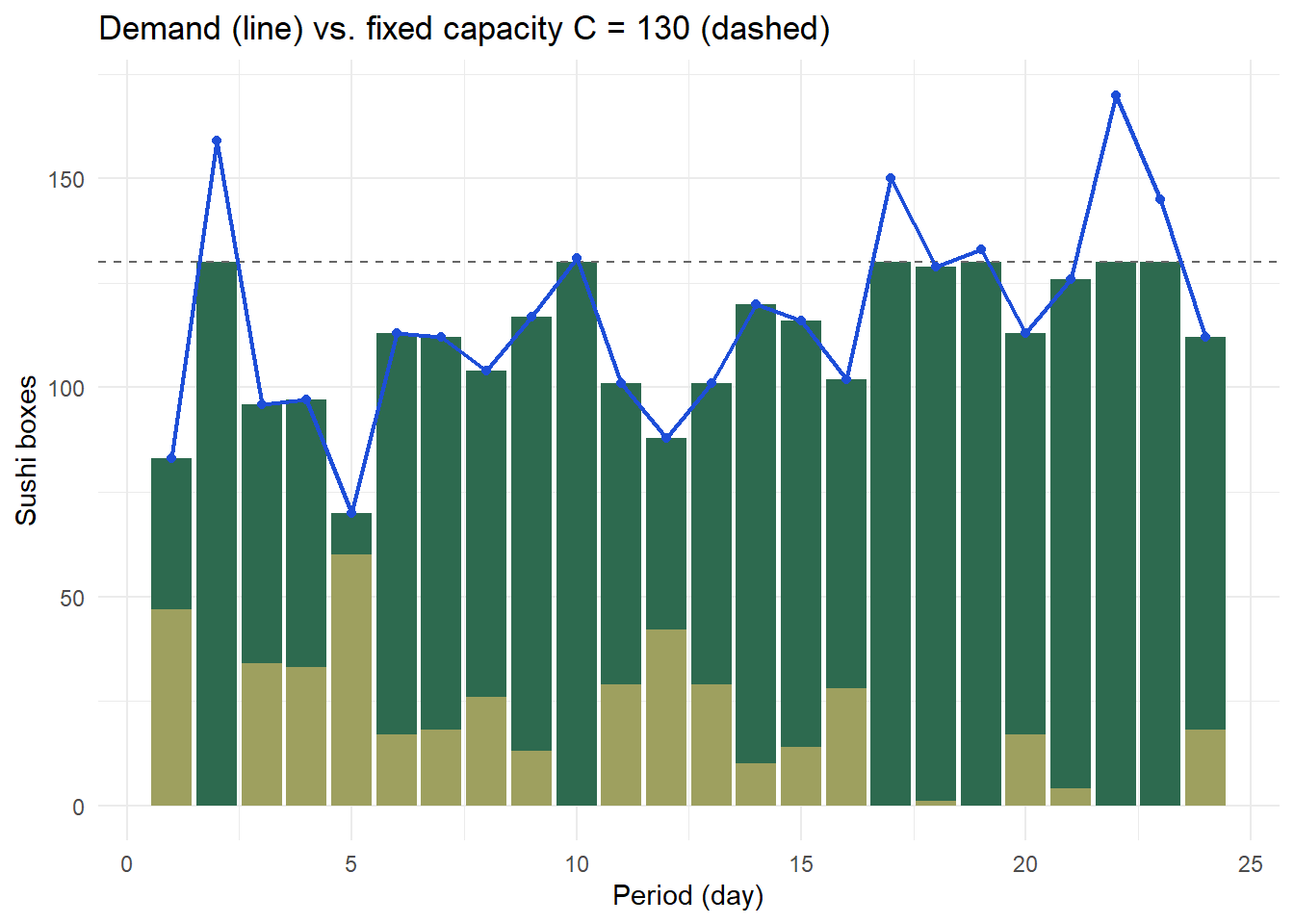
With this tool, the mismatch between capacity and demand described at the outset can be simulated directly. Suppose that production for the Wiesbaden store (central today) had — when, at an earlier expansion stage, it was still planned independently — a fixed capacity of $C = 130$ boxes per day, while actual demand fluctuates around this capacity, normally distributed with $\mu = 120$ and $\sigma = 25$:
```{r}
#| label: ch6-mismatch-sim
#| fig-cap: "Mismatch between fixed capacity and stochastic demand (Wiesbaden store)"
set.seed(12)             # reproducible simulation
n_perioden <- 24
C <- 130                 # fixed capacity (boxes/day)

demand_mismatch <- tibble(
  periode        = 1:n_perioden,
  # draw demand, round to integers, exclude negative values
  nachfrage      = pmax(40, round(rnorm(n_perioden, mu_d, sigma_d))),
  produktion     = pmin(nachfrage, C),        # actually sold
  fehlmenge      = pmax(0, nachfrage - C),    # lost sales
  leerkapazitaet = pmax(0, C - nachfrage)     # unused capacity
)

ggplot(demand_mismatch, aes(x = periode)) +
  # bars: production (dark) + idle capacity (light) up to the capacity limit
  geom_col(aes(y = produktion), fill = "#2D6A4F") +
  geom_col(aes(y = leerkapazitaet, group = 1), fill = "#E9C46A", alpha = 0.6,
           position = position_nudge(y = 0)) +
  geom_hline(yintercept = C, linetype = "dashed", color = "grey40") +
  geom_line(aes(y = nachfrage), color = "#1D4ED8", linewidth = 0.8) +
  geom_point(aes(y = nachfrage), color = "#1D4ED8") +
  labs(x = "Period (day)", y = "Sushi boxes",
       title = "Demand (line) vs. fixed capacity C = 130 (dashed)") +
  theme_minimal()
# Share of periods with a shortage and with idle capacity
mean(demand_mismatch$fehlmenge > 0)
mean(demand_mismatch$leerkapazitaet > 0)
```
Although the capacity of 130 boxes is clearly above the expected demand of 120 boxes, in this simulation run **shortages** occur on 25% of days and **idle capacity** on 75% of days — depending on whether the random realisation lies above or below the capacity limit. This is not the result of poor planning, but an unavoidable consequence of combining fixed capacity with stochastic demand. For a fresh product such as a sushi box, this weighs particularly heavily: idle capacity here means not only unused machine time but, in the case of overproduction, also **food waste**, while shortages lead directly to lost revenue and disappointed store partners. SushiFresh encounters exactly this dilemma elsewhere too: on public holidays with demand peaks, during sudden changes in the weather, or during short-term promotions at individual stores.
The central design question of this chapter is therefore: **how can this mismatch be reduced — without additional physical capacity?** One of the most effective answers is pooling.
## Capacity Pooling: Risk Pooling of Production Capacities
### Forms of Pooling at a Glance
The term **pooling** (also *risk pooling*) generally refers to the bundling of resources, inventories or demands so that random fluctuations offset one another. The literature typically distinguishes several forms [cf. @silver2017inventory, Ch. 6; @simchilevi2010operations]:
- **Location/inventory pooling**: several regional warehouses are merged into one central warehouse (focus of this chapter, see the section on inventory pooling — at SushiFresh, the consolidation of supply onto a single central kitchen, as suggested by Chapter [-@sec-standort-2]).
- **Capacity pooling**: several production facilities are made flexible so that they can stand in for one another (focus of the following section).
- **Product pooling**: several product variants are kept as a common, undifferentiated intermediate product for as long as possible and only given their final configuration late in the value creation process (*postponement*).
- **Capacity/component pooling through standardisation**: common parts or modules are used across several end products, so that their requirements are pooled in procurement (at SushiFresh, e.g. joint procurement of rice or nori for all box variants).
All of these variants follow the same basic statistical principle, which is derived formally in the rest of this chapter, first using the example of capacities and then of inventories. We begin with a look back at SushiFresh's start-up phase, long before the decision from Chapter [-@sec-standort-2] was made.
### Initial Situation: Two Pilot Kitchens, No Flexibility
In its start-up phase, SushiFresh initially supplied only two pilot locations — today's **Wiesbaden** and **Mainz** stores — each via its own small production kitchen on site [structure of the example cf. @cachon2024matching, Ch. 17]. Each kitchen was set up exclusively for its own location — there was **no technological flexibility**. Both kitchens had the same capacity $C^1 = C^2 = 90$ boxes per day. Over twelve (pilot) months, the following demands were observed:
```{r}
#| label: ch6-pooling-data
C1 <- C2 <- 90   # capacity per kitchen (boxes per day, pilot phase)

cp_data <- tibble(
  Monat = 1:12,
  dA    = c(78, 79, 92, 76, 95, 104, 87, 92, 91, 85, 96, 93),  # demand at Wiesbaden pilot location
  dB    = c(102, 92, 93, 87, 80, 97, 90, 76, 89, 86, 89, 93)   # demand at Mainz pilot location
)

# Without pooling: each kitchen serves only its own location,
# sales are capped from above by capacity
cp_data <- cp_data |>
  mutate(xA = pmin(dA, C1),
         xB = pmin(dB, C2))

# Mean demand, mean sales and utilisation per kitchen
cp_data |>
  summarise(E_dA = mean(dA), E_dB = mean(dB),
            E_xA = mean(xA), E_xB = mean(xB),
            Utilisation_1 = mean(xA) / C1, Utilisation_2 = mean(xB) / C2)
```
Both kitchens are well utilised at around 96–97%, and the fill rate (share of demand that is actually delivered) is already above 97%. Nevertheless, **in total over the year**, both shortages (when demand exceeds 90) and idle capacity (when it falls below) arise — a direct example of the structural mismatch described in the previous section, this time applied to two parallel pilot kitchens.
### One-Sided and Two-Sided Capacity Pooling
The decisive question is: can one kitchen help out when the other location is overloaded? Suppose the Wiesbaden kitchen is technically upgraded so that it can **also** produce boxes for Mainz in addition to its own location (**one-sided pooling**). As soon as demand in Mainz on a given day exceeds the capacity of the Mainz kitchen ($d^B_t > C^2$) and the Wiesbaden kitchen still has spare capacity ($d^A_t < C^1$), it steps in:
$$
x_t^{1} = d_t^A + \min\bigl(C^1 - d_t^A;\; d_t^B - C^2\bigr), \qquad x_t^{2B} = C^2
$$
```{r}
#| label: ch6-pooling-onesided
cp_pool_1 <- cp_data |>
  mutate(
    # The Wiesbaden kitchen first covers its own location and, if it has
    # spare capacity, additionally produces for Mainz
    x1A = pmin(dA, C1),
    x1B = ifelse(dB > C2 & dA < C1, pmin(C1 - dA, dB - C2), 0),
    x1  = x1A + x1B,
    x2B = pmin(C2, dB),
    xB  = x2B + x1B                 # total sales in Mainz
  )

cp_pool_1 |>
  summarise(Utilisation_Kitchen1 = mean(x1) / C1,
            ServiceLevel_Mainz   = mean(xB) / mean(dB))
```
The fill rate in Mainz already rises noticeably through this **one-sided** assistance. If, in addition, the Mainz kitchen is also allowed to step in for Wiesbaden when required (**two-sided pooling**), the separation between kitchens and locations is effectively removed:
```{r}
#| label: ch6-pooling-twosided
cp_pool <- cp_data |>
  mutate(
    x1A = pmin(dA, C1),
    x1B = ifelse(dB > C2 & dA < C1, pmin(C1 - dA, dB - C2), 0),
    x1  = x1A + x1B,
    x2B = pmin(C2, dB),
    x2A = ifelse(dA > C1 & dB < C2, pmin(C2 - dB, dA - C1), 0),
    x2  = x2A + x2B,
    xA  = x1A + x2A,
    xB  = x1B + x2B
  )

cp_pool |>
  summarise(Utilisation_1 = mean(x1) / C1, Utilisation_2 = mean(x2) / C2,
            ServiceLevel_Wiesbaden = mean(xA) / mean(dA),
            ServiceLevel_Mainz     = mean(xB) / mean(dB))
```
```{r}
#| label: ch6-kpi-table
#| tbl-cap: "KPI comparison: no pooling vs. one-sided vs. two-sided pooling (SushiFresh pilot phase)"
# Absolute lost sales over all 12 months, per scenario
kpi_df <- tibble(
  Kennzahl = c("Utilisation, Wiesbaden kitchen (%)", "Utilisation, Mainz kitchen (%)",
               "Sales ratio Wiesbaden (%)", "Sales ratio Mainz (%)",
               "Total lost sales (boxes)"),
  Dezentral = c(round(mean(cp_data$xA) / C1 * 100, 1),
                round(mean(cp_data$xB) / C2 * 100, 1),
                round(sum(cp_data$xA) / sum(cp_data$dA) * 100, 1),
                round(sum(cp_data$xB) / sum(cp_data$dB) * 100, 1),
                sum(cp_data$dA - cp_data$xA) + sum(cp_data$dB - cp_data$xB)),
  Pooling_einseitig = c(round(mean(cp_pool_1$x1) / C1 * 100, 1),
                round(mean(cp_pool_1$x2B) / C2 * 100, 1),
                round(sum(cp_pool_1$x1A) / sum(cp_data$dA) * 100, 1),
                round(sum(cp_pool_1$xB) / sum(cp_data$dB) * 100, 1),
                sum(cp_data$dA - cp_pool_1$x1A) + sum(cp_data$dB - cp_pool_1$xB)),
  Pooling_zweiseitig = c(round(mean(cp_pool$x1) / C1 * 100, 1),
                round(mean(cp_pool$x2) / C2 * 100, 1),
                round(sum(cp_pool$xA) / sum(cp_data$dA) * 100, 1),
                round(sum(cp_pool$xB) / sum(cp_data$dB) * 100, 1),
                sum(cp_data$dA - cp_pool$xA) + sum(cp_data$dB - cp_pool$xB))
)

kbl(kpi_df,
    col.names = c("KPI", "Decentralised", "Pooling (one-sided)", "Pooling (two-sided)"),
    align = c("l", "r", "r", "r")) |>
  kable_styling(bootstrap_options = c("condensed", "striped"), full_width = TRUE)
```
The pattern is clear: **capacity pooling improves all service metrics simultaneously** — higher utilisation, higher sales ratio, fewer lost sales — and it does so **without creating a single additional unit of production capacity**. The effect arises solely because positive and negative deviations of the two locations from their respective capacities partially offset each other: if Wiesbaden is lightly loaded and Mainz heavily loaded, the spare capacity of the Wiesbaden kitchen can flow to where it is needed. This **risk pooling effect** is the unifying principle that this chapter treats for capacities, for inventories and finally, formally, via the square-root law.
Pooling is not free, however: it requires **technological flexibility** (kitchens must be able to produce for several locations and reschedule between them just in time) and additional **logistical coordination**. It is ultimately precisely this cost–benefit trade-off — distributed, flexible capacity versus a single, efficient central plant — that also shapes SushiFresh's choice between one and several production sites (Chapter [-@sec-standort-2]). The more locations are to be integrated, the more complex and expensive flexibility becomes, which raises the question of how pooling can be organised sensibly across many locations without every location literally being able to stand in for every other.
### Chaining: Pooling Benefits Without Full Flexibility
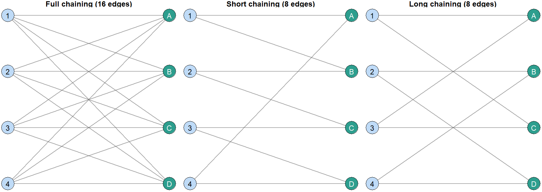
With $n$ plants and $n$ markets, **full pooling** would mean that every plant can supply every market — with four plants and four markets, that is $n \times n = 16$ possible plant–market links. In practice, this is usually uneconomical, because each plant would have to invest in every additional product technology. The surprising insight of pooling theory [cf. @cachon2024matching, Ch. 17], however, is: **you do not have to pool fully to obtain almost the full benefit.** It is sufficient to connect the plants and markets into a **chain**, in which each plant can serve exactly two markets and each market can be served by exactly two plants:
```{r}
#| label: ch6-chaining-diagram
#| fig-cap: "Three chaining strategies compared: full, short and long chaining"
#| fig-width: 9
#| fig-height: 3.2
plants  <- tibble(id = paste0("Werk ", 1:4), lbl = as.character(1:4), x = 0, y = c(4, 3, 2, 1))
markets <- tibble(id = LETTERS[1:4], lbl = LETTERS[1:4], x = 1, y = c(4, 3, 2, 1))

# Full chaining: every plant connected to every market (n x n edges)
edges_full <- expand_grid(from = plants$id, to = markets$id) |>
  mutate(chaining = "Full chaining (16 edges)")

# Short chaining: each plant serves its "own" market plus its direct
# neighbour in the ring (2 edges per plant, 2n edges in total)
edges_short <- tibble(
  from     = rep(plants$id, 2),
  to       = c(markets$id, markets$id[c(2, 3, 4, 1)]),
  chaining = "Short chaining (8 edges)"
)

# Long chaining: like short chaining, but the second market is two positions
# further along the ring -> more market coverage per plant with the same number of edges
edges_long <- tibble(
  from     = rep(plants$id, 2),
  to       = c(markets$id, markets$id[c(3, 4, 1, 2)]),
  chaining = "Long chaining (8 edges)"
)

edges_all <- bind_rows(edges_full, edges_short, edges_long) |>
  left_join(plants  |> rename(x0 = x, y0 = y), by = c("from" = "id")) |>
  left_join(markets |> rename(x1 = x, y1 = y), by = c("to"   = "id")) |>
  mutate(chaining = factor(chaining, levels = c("Full chaining (16 edges)",
                                                 "Short chaining (8 edges)",
                                                 "Long chaining (8 edges)")))

ggplot(edges_all) +
  geom_segment(aes(x = x0, y = y0, xend = x1, yend = y1),
               color = "grey40", alpha = 0.55,
               arrow = arrow(length = unit(0.12, "cm"))) +
  geom_point(data = plants,  aes(x = x, y = y), size = 7, shape = 21, fill = "#BFDBF7") +
  geom_point(data = markets, aes(x = x, y = y), size = 7, shape = 21, fill = "#2D9E8E") +
  geom_text(data = plants,  aes(x = x, y = y, label = lbl), size = 3) +
  geom_text(data = markets, aes(x = x, y = y, label = lbl), size = 3, color = "white") +
  facet_wrap(~chaining) +
  theme_void() +
  theme(strip.text = element_text(face = "bold", size = 9))
```
With **short chaining**, each plant serves its own market as well as the directly neighbouring market in the ring; with **long chaining**, the second market served lies two positions further away. Both variants require only $2n$ instead of $n^2$ links — with four plants, 8 instead of 16 — yet empirically achieve a large share of the pooling benefit of full flexibility, because a local demand surplus can be passed along the chain to the next plant with spare capacity. This principle — which became known as **chaining** through General Motors' plant allocation practice — is an example of the fact that the marginal benefit of additional flexibility **diminishes sharply**: the first few additional links deliver most of the pooling effect, while full flexibility adds only a small further gain at sharply rising costs.
For a company such as SushiFresh with six stores, chaining would have been a conceivable intermediate solution — for instance, several smaller regional kitchens, each of which can supply two neighbouring stores. If the company instead opts for full centralisation at a single site, this does not refute the chaining principle, but is the result of a concrete cost–benefit trade-off: given the short distances in the Rhine-Main area and relatively low additional costs for central logistics, the full pooling benefit outweighs the consolidation costs. For more widely distributed networks or with high transport costs, this trade-off often turns out differently — partial flexibility such as chaining is then the more economical choice. The (diminishing) marginal benefit of additional links must always be weighed against the (usually linearly or even progressively rising) marginal costs of additional changeover capability — a classic cost–benefit trade-off, as already familiar from the discussion of trade-offs in Chapter [-@sec-logistikkosten].
## Safety Stocks: Reorder Policies and Service Level
Pooling works not only between parallel locations but also **over time**: safety stocks offset demand fluctuations within a replenishment lead time. Before the pooling effect for inventories is discussed, we first need to clarify how a safety stock is dimensioned in the first place.
### The Periodic Review (t, S) Policy
A widely used inventory control method is the **periodic order-up-to policy** — also called the $(t, S)$ policy: at fixed intervals $t$, the current **inventory position** (physical stock plus orders already placed but not yet received, minus shortages) is raised to a fixed **target level** $S$ (*order-up-to level*). Between placing an order and receiving the goods, the **replenishment lead time** $wbz$ always elapses. The **safety stock** $sb$ is the difference between this target level and the expected demand during the *risk period* (review interval plus replenishment lead time):
$$
sb = S - \mu \cdot (t + wbz)
$$
where $\mu$ is the expected demand per period. The further $S$ lies above this expected demand, the larger the buffer against positive demand spikes — but the higher the capital tied up as well. If, within the risk period, more demand actually occurs than the available stock can cover, a **shortage** arises: depending on how the company deals with it, a distinction is made between **backorders** (demand is delayed but delivered in full as soon as stock is available again) and **lost sales** (unmet demand is irretrievably lost). The two cases differ in how net inventory is updated: with backordering, net inventory may temporarily become negative; with lost sales, it is bounded below by zero.
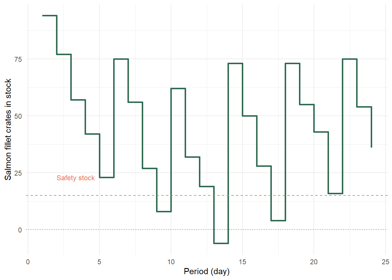
At SushiFresh, this policy does not apply to the finished sushi boxes themselves (which, as mentioned, can hardly be stored), but to **raw material procurement** at the central kitchen in Raunheim: fresh salmon fillet is ordered from a fish wholesaler not daily but periodically, and held in cold storage for a short time. The simulation functions `simuliere_tS()` and `tS.lager()` in `R/scm_functions.R` replicate exactly this logic: period by period, they update demand, orders, deliveries and the resulting stock, explicitly distinguishing between physical stock, net inventory and inventory position (physical stock plus orders already placed but not yet received). How this updating works in detail does not need to be rebuilt here — what matters is being able to interpret the **result**:
```{r}
#| label: ch6-ts-lager-sim
#| fig-cap: "Simulated salmon fillet stock at the Raunheim central kitchen under a (t, S) policy"
set.seed(42)                      # reproducible demand draws
n     <- 24                       # simulation horizon (periods = days)
lam   <- 20                       # mean daily consumption of salmon fillet crates (Poisson-distributed)
t     <- 4                        # review interval with the fish wholesaler (days)
S     <- 135                      # order-up-to level (crates)
wbz   <- 2                        # replenishment lead time (days)
l.ini <- 120                      # initial stock (crates)

sb <- S - (t + wbz) * lam         # safety stock according to the formula above
sb
# Draw period demands (Poisson fits discrete crate quantities well)
verbrauch <- rpois(n, lambda = lam)

# Apply the ready-made simulation function from scm_functions.R
res <- tS.lager(d = verbrauch, t = t, S = S, l.ini = l.ini, wbz = wbz) |>
  as_tibble() |>
  mutate(Periode = row_number())

ggplot(res, aes(x = Periode, y = Lagerbestand)) +
  geom_step(color = "#2D6A4F", linewidth = 0.9) +
  geom_hline(yintercept = sb, linetype = "dashed", color = "#E76F51") +
  geom_hline(yintercept = 0, linetype = "dotted", color = "grey50") +
  annotate("text", x = 2, y = sb + 8, label = "Safety stock", color = "#E76F51",
           hjust = 0, size = 3.2) +
  labs(x = "Period (day)", y = "Salmon fillet crates in stock") +
  theme_minimal()
# Minimum stock over the simulation horizon
min(res$Lagerbestand)
```
In this simulation, the salmon fillet stock briefly drops below zero in period 13 — despite a calculated safety stock of 15 crates, a **shortage** occurs, because the consumption actually drawn was above the mean on several consecutive days. This already illustrates the central point: a safety stock based on the *expected value* does **not guarantee** protection against shortages, but only protects **with a certain probability**. This probability must be chosen explicitly — which leads to the concept of the service level.
::: {.vertiefung}
**In depth (theory): Normal distribution, z-transformation and quantiles**
Many formulas in this and the following chapters are based on the normal distribution. Its **density function** $f(x) = \frac{1}{\sigma\sqrt{2\pi}} \exp\!\left(-\frac{(x-\mu)^2}{2\sigma^2}\right)$ describes how the probability mass is distributed around the mean $\mu$; the **distribution function** $F(x) = P(X \leq x) = \int_{-\infty}^x f(t)\,dt$ gives the cumulative probability. Three properties are central in practice:
1. **68–95–99.7 rule:** around 68.3% of the probability mass lies in the interval $\mu \pm \sigma$, around 95.4% in $\mu \pm 2\sigma$ and around 99.7% in $\mu \pm 3\sigma$.
2. **z-transformation:** every normally distributed random variable $X \sim \mathcal{N}(\mu,\sigma^2)$ can be transformed into the **standard normal distribution** $\mathcal{N}(0,1)$ via $Z = (X-\mu)/\sigma$. It holds that $P(X \leq x) = \Phi\big((x-\mu)/\sigma\big)$, where $\Phi$ is the distribution function of the standard normal distribution. A single table (or the R function `pnorm()`) is therefore sufficient for all normal distributions.
3. **Symmetry:** $\Phi(-z) = 1 - \Phi(z)$; a table for $z \geq 0$ is therefore sufficient.
The inverse yields the **quantile** $z_\alpha = \Phi^{-1}(\alpha)$ (in R: `qnorm(alpha)`): the value that is not exceeded with probability $\alpha$. From $P(D \leq S) = \alpha$ it follows that $S = \mu + z_\alpha\,\sigma$ and hence the safety stock $sb = z_\alpha \cdot \sigma$. The most important values:
```{r}
#| label: ch6-z-tabelle
tibble(service_level = c(0.90, 0.95, 0.975, 0.99, 0.999),
       z_alpha = round(qnorm(service_level), 3))
```
Example from the lecture: with $D \sim \mathcal{N}(500, 80^2)$ and $\alpha = 95\,\%$, we obtain $sb = 1.645 \cdot 80 \approx 132$ units. Intuitively: anyone wishing to raise their service level from 95% to 99% must increase the safety stock by a factor of $2.326/1.645 \approx 1.41$ – the last percentage points of availability are particularly expensive because of the thin tails of the distribution.
:::
### The $\alpha$ Service Level and the Empirical Distribution Function
The **$\alpha$ service level** (also *cycle service level*) is defined as the probability of **not** suffering a shortage during the risk period:
$$
\alpha = P(D \leq S)
$$
Here, $D$ is the (random) demand during the risk period and $S$ the stock available at its start. The $\alpha$ service level is an **event probability**: it answers the question "How often, across many risk periods, does no shortage at all occur?" — regardless of how large a shortage is when one does occur. In addition, the **$\beta$ service level** (*fill rate*) is also frequently used in practice; it instead measures the **quantity-based** share of demand that can be served directly from stock: $\beta = 1 - E[\text{shortage}]/E[\text{demand}]$. A high $\alpha$ service level does not rule out rare but large shortages — for most operational purposes, however, $\alpha$ is the more common and more easily communicated metric, which is why it is the focus in what follows. If the distribution of $D$ is unknown, $\alpha$ can be estimated directly from historical observations — via the **empirical distribution function**.
::: {.r-exkurs}
**R aside: The empirical distribution function with `ecdf()`**
For a sample $x_1, \dots, x_n$, the empirical cumulative distribution function (ECDF) gives the **share** of observations that are less than or equal to a value $x$:
$$
\hat{F}(x) = \frac{1}{n}\sum_{i=1}^{n} \mathbb{1}(x_i \leq x)
$$
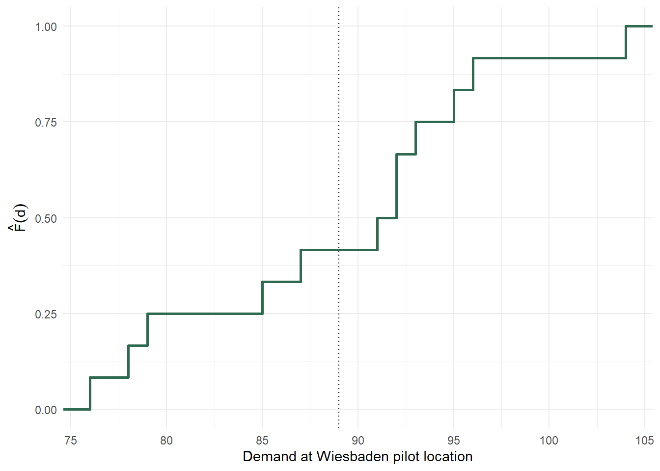
In R, `ecdf(x)` returns this function not as a table but as a **callable R object** — so it can be evaluated like a function at any point:
```{r}
#| label: ch6-ecdf-demo
#| fig-cap: "Empirical distribution function of demand at the Wiesbaden pilot location"
F_A <- ecdf(cp_data$dA)      # ECDF object from the 12 monthly pilot values for Wiesbaden

# F_A can be called like any other function:
F_A(90)                      # share of months with demand <= 90
ggplot(cp_data, aes(x = dA)) +
  stat_ecdf(geom = "step", color = "#2D6A4F", linewidth = 0.9) +
  geom_vline(xintercept = mean(cp_data$dA), linetype = "dotted") +
  labs(x = "Demand at Wiesbaden pilot location", y = expression(hat(F)(d))) +
  theme_minimal()
```
The inverse — "which value is not exceeded with probability $\alpha$?" — is provided by `quantile(x, probs = alpha)`. This allows the stock level matching a desired service level to be read **directly from the data**, without any distributional assumption.
:::
Formally: we are looking for the smallest stock level $S$ for which $\hat{F}(S) \geq \alpha$ — i.e. the empirical $\alpha$-quantile $S = \hat{F}^{-1}(\alpha)$. For the demand data of the Wiesbaden pilot location, we obtain:
```{r}
#| label: ch6-alpha-quantile
alpha_niveaus <- c(0.75, 0.90, 0.95)

sb_tabelle <- tibble(
  alpha = alpha_niveaus,
  # empirical quantile per service level (type 1: "next largest observation")
  S     = map_dbl(alpha_niveaus, ~ quantile(cp_data$dA, probs = .x, type = 1))
) |>
  mutate(sb = S - mean(cp_data$dA))   # safety stock = quantile minus mean

sb_tabelle
```
A service level of 75% thus requires only 4 boxes of safety stock, whereas a service level of 95% already requires 15 boxes. This strongly **disproportionate** relationship — the last percentage points of service level are disproportionately expensive — is a direct consequence of the shape of the demand distribution, and we will encounter it again in a similar form in the newsvendor model in @sec-newsvendor (there again using the example of the Frankfurt store).
## Inventory Pooling: Risk Pooling Across Locations
### Decentralised vs. Centralised Inventory Holding
The decisive question now is: what happens to the required safety stock if the two pilot locations Wiesbaden and Mainz are supplied **not** from separate kitchens but from a **shared central plant**? In the decentralised case, each location must hold its own safety stock — in total, therefore, $sb_{Wiesbaden} + sb_{Mainz}$. In the centralised case, a single safety stock for the **aggregated** demand $D_0 = D_{Wiesbaden} + D_{Mainz}$ is sufficient:
```{r}
#| label: ch6-pooling-ecdf-vergleich
alpha <- 0.95

# Decentralised: safety stock per location, then summed
S_A <- quantile(cp_data$dA, alpha, type = 1);  sb_A <- S_A - mean(cp_data$dA)
S_B <- quantile(cp_data$dB, alpha, type = 1);  sb_B <- S_B - mean(cp_data$dB)
sb_dezentral <- sb_A + sb_B

# Centralised: one safety stock for the total demand Wiesbaden + Mainz
dTotal <- cp_data$dA + cp_data$dB
S_T    <- quantile(dTotal, alpha, type = 1)
sb_zentral <- S_T - mean(dTotal)

tibble(Configuration = c("Decentralised (Wiesbaden + Mainz separate)", "Centralised (pooled)"),
       Safety_stock = c(sb_dezentral, sb_zentral),
       Saving_percent = c(0, round((1 - sb_zentral / sb_dezentral) * 100, 1)))
```
Merely by merging the two pilot kitchens, the required safety stock falls by around 18% — with an **identical** stockout probability of 5%. This effect is not based on additional information or better forecasting, but purely on a statistical principle: random deviations of individual locations from their mean partially offset one another in the **sum**, as long as demands are not perfectly positively correlated.
### Formal Derivation for Normally Distributed Demand
To capture this effect algebraically, let the demands at two locations be normally distributed: $D_1 \sim \mathcal{N}(\mu_1, \sigma_1^2)$ and $D_2 \sim \mathcal{N}(\mu_2, \sigma_2^2)$, with correlation $\rho = \text{Cor}(D_1, D_2)$. The safety stock at decentralised location $i$ at service level $\alpha$ is $sb_i = z_\alpha \cdot \sigma_i$ in each case (with $z_\alpha = \Phi^{-1}(\alpha) =$ `qnorm(alpha)`), giving a total of:
$$
sb_{dez} = z_\alpha \cdot (\sigma_1 + \sigma_2)
$$
For the sum of two (jointly) normally distributed random variables, a theorem from probability theory applies: the sum is again normally distributed, with a variance that also takes into account the covariance between $D_1$ and $D_2$:
$$
D_0 = D_1 + D_2 \sim \mathcal{N}\!\left(\mu_1 + \mu_2,\; \sigma_1^2 + \sigma_2^2 + 2\rho\,\sigma_1\sigma_2\right)
$$
The central safety stock is therefore:
$$
sb_{zen} = z_\alpha \cdot \sqrt{\sigma_1^2 + \sigma_2^2 + 2\rho\,\sigma_1\sigma_2}
$$
The decisive comparison is $sb_{zen}$ versus $sb_{dez}$ as a function of $\rho$. Three limiting cases illustrate the range:
| Correlation | Central safety stock |
|:---:|:---|
| $\rho = -1$ (perfectly opposed) | $z_\alpha \cdot \lvert \sigma_1 - \sigma_2 \rvert$ |
| $\rho = 0$ (uncorrelated) | $z_\alpha \cdot \sqrt{\sigma_1^2 + \sigma_2^2}$ |
| $\rho = +1$ (perfectly aligned) | $z_\alpha \cdot (\sigma_1 + \sigma_2) = sb_{dez}$ |
Since $\lvert \sigma_1 - \sigma_2\rvert \leq \sqrt{\sigma_1^2+\sigma_2^2} \leq \sigma_1+\sigma_2$ always holds for non-negative $\sigma_1, \sigma_2$, it follows that: **pooling always pays off as long as $\rho < 1$ — and the benefit is greater the more negative the correlation.** Only if both locations fluctuate in exactly the same direction ($\rho = +1$) does pooling bring no advantage at all, because no offsetting can then take place.
This formula can be generalised directly to more than two locations: for $n$ locations with individual $\sigma_i$ and (in the independent case) $\rho_{ij} = 0$ for all $i \neq j$, simply $sb_{zen} = z_\alpha \cdot \sqrt{\sum_i \sigma_i^2}$. It is precisely this generalisation that is applied in the next section to **SushiFresh's core business** — the six real stores.
### Application: The Safety Stock for the Six SushiFresh Stores
With a consolidation as suggested by Chapter [-@sec-standort-2], no longer just two pilot locations but all **six stores** are supplied from a single central kitchen in Raunheim. For each store, daily demand is approximately normally distributed, with the following parameters (estimated from sales data):
```{r}
#| label: ch6-sushifresh-filialen
filialen <- tibble(
  Filiale = c("Wiesbaden", "Mainz", "Frankfurt", "Rüsselsheim", "Darmstadt", "Offenbach"),
  mu      = c(120, 150, 280, 90, 110, 95),
  sigma   = c(25, 30, 55, 20, 24, 22)
)

filialen |>
  summarise(Stores = n(), Total_demand = sum(mu), Sum_sigma = sum(sigma))
```
Frankfurt is by far the largest **and** most volatile store — with $\mu = 280$ and $\sigma = 55$, it accounts for just under a third of total demand, but also for almost a third of total dispersion. The central question now is: how high is the safety stock in a central kitchen for a target service level of $\alpha = 95\,\%$ — compared with the hypothetical case in which each store continued to plan its replenishment independently? Under the (for now simplifying) assumption of independent store demands ($\rho_{ij} = 0$), this can be calculated directly with `qnorm()`:
```{r}
#| label: ch6-sushifresh-kernergebnis
alpha  <- 0.95
z_a    <- qnorm(alpha)          # critical z-value, verified with qnorm()
z_a
# Decentralised: sum of the individual safety stocks
sb_dezentral_sf <- z_a * sum(filialen$sigma)
sb_dezentral_sf
# Centralised (pooled, independence assumption): square root of the sum of variances
sigma_gepoolt <- sqrt(sum(filialen$sigma^2))
sigma_gepoolt
sb_zentral_sf <- z_a * sigma_gepoolt
sb_zentral_sf
# Relative saving through centralisation
einsparung_sf <- (1 - sb_zentral_sf / sb_dezentral_sf) * 100
round(c(decentralised = sb_dezentral_sf, centralised = sb_zentral_sf, saving_pct = einsparung_sf), 1)
```
The result is clear: if each store had to hold its own safety stock, **289.5 boxes** would be needed. In a shared central kitchen, by contrast, **127.5 boxes** are sufficient to achieve the same 95% service level — a **reduction of 56.0%**. As a cross-check of the formula derived by hand, the generic function of the same name, `pooling_safety_stock()`, from `R/scm_functions.R` can be used — albeit with one important limitation: it assumes $n$ **identical** locations with a common $\sigma$, whereas the SushiFresh stores differ in size and volatility. As an approximate cross-check, we can therefore examine what central safety stock the function would return for $n = 6$ locations with the **average** dispersion:
```{r}
#| label: ch6-sushifresh-gegenprobe
sigma_mean <- mean(filialen$sigma)   # 176 / 6 = 29.33 -- "average" store
sigma_mean
# Idealised comparison case: 6 identical stores with sigma = sigma_mean
ideal_fall <- pooling_safety_stock(n = 6, sigma = sigma_mean, z = z_a)
ideal_fall
```
The idealised comparison case (six **identical** stores with $\sigma = 29.33$) yields a saving of `r round((1 - qnorm(0.95)*sqrt(6)*mean(c(25,30,55,20,24,22)) / (qnorm(0.95)*6*mean(c(25,30,55,20,24,22))))*100,1)`% — remarkably, **more** than the 56.0% actually calculated for the real, heterogeneous SushiFresh stores. This may come as a surprise at first, but follows directly from a mathematical property: for a **fixed sum** $\sum_i \sigma_i$, the sum of squares $\sum_i \sigma_i^2$ is **minimal** when all $\sigma_i$ are equal (a direct consequence of the inequality between the quadratic and arithmetic means). Any deviation from this equal distribution — such as the dominant, above-average volatile Frankfurt store with $\sigma = 55$ — **increases** $\sum_i \sigma_i^2$ compared with the idealised case, and thus also the pooled safety stock $\sigma_{zen}$. The pooling **benefit** is therefore greatest when many **similarly sized** locations are pooled; a single, dominant outlier location such as Frankfurt "dilutes" the relative diversification advantage, because it spreads the overall risk less evenly across the six locations than the ideal assumption presumes. This insight matters for facility location planning: a network of **many similarly sized** stores benefits relatively more from pooling than a network with one dominant large location.
::: {.callout-note}
The two figures of 289.5 and 127.5 boxes are the safety stock **in addition** to the expected demand of 845 boxes/day (see the store table above). They thus quantify exactly the effect that centralisation has on the capital tied up in safety stock — independently of the location and transport costs (treated in Chapters [-@sec-standort-1] and [-@sec-standort-2]).
:::
::: {.fallstudie}
**Case study: What is the pooling saving worth to SushiFresh?**
Chapter [-@sec-standort-2] showed that the cost differences between a central kitchen in Raunheim and a two-site solution (Raunheim + Wiesbaden-Erbenheim) amount to only around €7,000 per year in the numerical example. Can the pooling effect be translated into the same currency? For fresh produce, "safety stock" means nothing other than **deliberate overproduction**, part of which remains unsold in the evening. The expected leftover quantity for a production quantity $q = \mu + z\,\sigma$ can be calculated with the normal loss function from Chapter [-@sec-newsvendor]: $E[(q-D)^+] = \sigma \cdot \big(\varphi(z) + z\,\Phi(z)\big)$. With overage costs of €3 per unsold box (Chapter [-@sec-newsvendor]), we obtain:
```{r}
#| label: ch6-pooling-wert
z   <- qnorm(0.95)
L_minus <- dnorm(z) + z * pnorm(z)          # E[(q-D)^+] / sigma at q = mu + z*sigma
c_o <- 3                                    # EUR per unsold box

rest_dezentral <- sum(filialen$sigma) * L_minus     # sum over six stores
rest_zentral   <- sigma_gepoolt * L_minus           # one pooled demand

tibble(
  Variant = c("Decentralised (each store separately)", "Centralised (pooled)"),
  Leftover_boxes_per_day = round(c(rest_dezentral, rest_zentral), 1),
  Cost_EUR_per_year      = round(c(rest_dezentral, rest_zentral) * c_o * 365)
)
```
The difference is well over a hundred thousand euros per year and exceeds the €7,000 cost difference from the location model many times over. Even a few unsold boxes saved per day (€7,000 / 365 days / €3 ≈ 6–7 boxes) would be enough to justify centralisation. One important limitation applies, however: the full effect only arises if the central kitchen can allocate the boxes to the stores **after** observing store demand – for instance through a second run at midday on which goods are replenished. If, on the other hand, all boxes are firmly allocated to the stores in the morning, each store must be buffered individually, and the pooling effect is reduced to the upstream raw materials (fish, rice), which are planned jointly in the central kitchen. The organisation of distribution therefore determines how much of the theoretical pooling benefit is actually realised – a good example of the interplay between strategic location choice and operational control.
:::
### Correlation Effects: When Stores Are Not Independent
The calculation so far assumes **independent** store demands. In practice, this is rarely met exactly: geographically neighbouring stores often share **common demand drivers** — such as the same weather, the same public holiday calendar or regional events. Wiesbaden and Mainz, for example, are separated only by the Rhine; Frankfurt and Offenbach border each other directly. How strongly does such a **positive correlation** weaken the pooling effect?
::: {.r-exkurs}
**R aside: Simple Monte Carlo simulation with `replicate()`**
A **Monte Carlo simulation** answers an analytically tedious or unknown question by **repeating** the underlying random experiment **very many times** and averaging the metric of interest over all repetitions. In R, `replicate(n, expression)` takes care of the repetition loop: it evaluates `expression` `n` times and collects the results — a more compact alternative to an explicit `for` loop with manual storage of results.
First, we need a helper function that generates two **correlated** normally distributed demands. The standard trick for this: from two *independent* standard normal variables $z_1, z_2$, a variable correlated with $z_1$ can be constructed as $z_1' = \rho\, z_1 + \sqrt{1-\rho^2}\, z_2$ — its correlation with $z_1$ is exactly $\rho$.
```{r}
#| label: ch6-monte-carlo-korrelation
# Generates n periods of correlated demand at two locations
simuliere_pooled_demand <- function(n, mu1, mu2, sigma1, sigma2, rho) {
  z1 <- rnorm(n)                             # independent standard normal variable
  z2 <- rho * z1 + sqrt(1 - rho^2) * rnorm(n)  # variable correlated with z1 (correlation = rho)
  tibble(
    d1 = mu1 + sigma1 * z1,
    d2 = mu2 + sigma2 * z2,
    d0 = d1 + d2                             # pooled (central) demand
  )
}

set.seed(2026)

# Monte Carlo simulation: Wiesbaden and Mainz, geographical neighbours with
# assumed correlation rho = 0.3 (e.g. shared weather/public holidays).
# Simulate 30 days 1000 times, each time determining the empirical safety stock
# of the POOLED demand at alpha = 95%
sb_mc <- replicate(1000, {
  sim <- simuliere_pooled_demand(n = 30, mu1 = 120, mu2 = 150,
                                  sigma1 = 25, sigma2 = 30, rho = 0.3)
  quantile(sim$d0, 0.95) - mean(sim$d0)
})

mean(sb_mc)                                                    # Monte Carlo estimator
qnorm(0.95) * sqrt(25^2 + 30^2 + 2 * 0.3 * 25 * 30) # analytical value for comparison
```
The simulated safety stock averaged over 1000 repetitions lies in the expected order of magnitude of the analytically calculated value — the residual deviation (caused by the small sample of 30 days per repetition) is a known property of quantile estimators and **confirms** the formula without the normality assumption having to be plugged explicitly into a closed-form solution. This approach is particularly valuable when (as in the last section of this chapter) the actual distribution deviates from the normal distribution and no closed-form formula exists any more.
:::
The direct comparison shows the effect of the correlation between Wiesbaden and Mainz particularly clearly: without correlation ($\rho = 0$), the central safety stock of both stores would be $z_\alpha\sqrt{25^2+30^2} \approx$ `r round(qnorm(0.95)*sqrt(25^2+30^2),1)` boxes; with the assumed correlation of $\rho = 0.3$, it rises to around `r round(qnorm(0.95)*sqrt(25^2+30^2+2*0.3*25*30),1)` boxes — the pooling advantage over $sb_{dez} =$ `r round(qnorm(0.95)*(25+30),1)` boxes shrinks from `r round((1-sqrt(25^2+30^2)/(25+30))*100,1)`% to only `r round((1-sqrt(25^2+30^2+2*0.3*25*30)/(25+30))*100,1)`%.
The same logic can be transferred to the **entire six-store network** — using `MASS::mvrnorm()` for multivariate, correlated normal distributions. Suppose that neighbouring pairs of stores are each correlated with $\rho = 0.3$ (Wiesbaden–Mainz, Frankfurt–Offenbach, Rüsselsheim–Darmstadt), while all other pairs remain uncorrelated:
```{r}
#| label: ch6-mvrnorm-korrelation-netzwerk
#| message: false
# Correlation matrix: 1 on the diagonal, 0.3 for the three neighbouring pairs
R_mat <- diag(6)
nachbarpaare <- list(c(1, 2), c(3, 6), c(4, 5))   # (Wiesbaden,Mainz), (Frankfurt,Offenbach), (Ruesselsheim,Darmstadt)
for (paar in nachbarpaare) R_mat[paar[1], paar[2]] <- R_mat[paar[2], paar[1]] <- 0.3
rownames(R_mat) <- colnames(R_mat) <- filialen$Filiale
R_mat
# Covariance matrix = correlation matrix scaled by the sigma values
Sigma_mat <- outer(filialen$sigma, filialen$sigma) * R_mat

# Analytical central safety stock under correlation:
# Var(sum) = sum of all entries of the covariance matrix
sb_zentral_korreliert <- z_a * sqrt(sum(Sigma_mat))
sb_zentral_korreliert
# Monte Carlo cross-check with MASS::mvrnorm()
set.seed(2026)
sim_netzwerk <- MASS::mvrnorm(n = 100000, mu = filialen$mu, Sigma = Sigma_mat)
d0_netzwerk  <- rowSums(sim_netzwerk)
sb_mc_netzwerk <- quantile(d0_netzwerk, 0.95) - mean(d0_netzwerk)
sb_mc_netzwerk
# Pooling saving with vs. without neighbourhood correlation
tibble(
  Scenario = c("Independent (rho = 0)", "Neighbouring stores correlated (rho = 0.3)"),
  SS_central = c(sb_zentral_sf, sb_zentral_korreliert),
  Saving_percent = c(round(einsparung_sf, 1),
                          round((1 - sb_zentral_korreliert / sb_dezentral_sf) * 100, 1))
)
```
Analytical formula and Monte Carlo simulation also agree very well in the six-dimensional case. In substantive terms: as soon as geographically neighbouring stores are positively correlated, the pooling saving falls from 56.0% to around 51% — risk pooling therefore still works, but noticeably less strongly, because part of the seemingly "random" demand fluctuations in fact has common causes that cannot be offset (e.g. a rainy weekend affects demand in Wiesbaden and Mainz at the same time). The practical implication is: when estimating the pooling benefit, the correlation structure between the merged locations should not be ignored — it can be estimated directly from historical sales data (`cor()`) and plugged into the covariance matrix above.
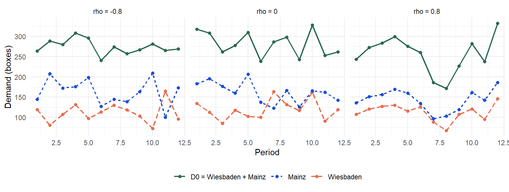
The following figure illustrates the correlation effect once more using three simulated demand paths for Wiesbaden and Mainz with identical marginal distributions but different correlations:
```{r}
#| label: ch6-korrelation-zeitreihen
#| fig-cap: "Pooled demand D0 = Wiesbaden + Mainz under different correlations"
#| fig-width: 9
#| fig-height: 3.4
set.seed(43)
rho_werte <- c(-0.8, 0, 0.8)

sim_rho <- map_dfr(rho_werte, function(rho) {
  simuliere_pooled_demand(12, 120, 150, 25, 30, rho) |>
    mutate(periode = row_number(), rho_label = paste0("rho = ", rho))
})

sim_rho_long <- sim_rho |>
  pivot_longer(cols = c(d1, d2, d0), names_to = "reihe", values_to = "wert") |>
  mutate(reihe = recode(reihe, d1 = "Wiesbaden", d2 = "Mainz", d0 = "D0 = Wiesbaden + Mainz"))

ggplot(sim_rho_long, aes(x = periode, y = wert, color = reihe, linetype = reihe)) +
  geom_line(linewidth = 0.8) +
  geom_point(size = 1.6) +
  facet_wrap(~rho_label) +
  scale_color_manual(values = c("Wiesbaden" = "#E76F51", "Mainz" = "#1D4ED8", "D0 = Wiesbaden + Mainz" = "#2D6A4F")) +
  labs(x = "Period", y = "Demand (boxes)", color = NULL, linetype = NULL) +
  theme_minimal() +
  theme(legend.position = "bottom")
```
With **negative** correlation ($\rho = -0.8$), the sum curve $D_0$ runs noticeably more smoothly than either of the two individual series — upward spikes in Wiesbaden tend to coincide with downward spikes in Mainz and cancel each other out. With **positive** correlation ($\rho = +0.8$), by contrast, the fluctuations reinforce each other, and $D_0$ fluctuates visibly more. Precisely this difference in the *smoothness* of the sum series is the intuitive counterpart of the formula derived above.
## The Square-Root Law of Pooling
The derivation so far applied to locations with potentially different dispersion and correlation. A particularly common and instructive special case arises when $n$ **identical, independent** locations are pooled — each with the same dispersion $\sigma$ and $\rho = 0$ between them. This case leads to the famous **square-root law of pooling** [cf. @simchilevi2010operations; @silver2017inventory, Ch. 6].
### Derivation
With $n$ independent, identically distributed locations with dispersion $\sigma$, the **decentralised** total safety stock is simply the sum of the $n$ individual stocks:
$$
sb_{dez} = n \cdot z_\alpha \cdot \sigma
$$
For the **centralised** variant, under independence ($\rho = 0$), the variances of the $n$ locations add up to a total variance of $n \cdot \sigma^2$. The standard deviation of the pooled demand is consequently **not** $n\sigma$, but only:
$$
\sigma_{zen} = \sqrt{n \cdot \sigma^2} = \sqrt{n}\cdot \sigma
$$
and therefore
$$
sb_{zen} = z_\alpha \cdot \sqrt{n}\cdot \sigma
$$
The ratio of the two safety stocks is remarkably simple:
$$
\frac{sb_{zen}}{sb_{dez}} = \frac{z_\alpha \sqrt{n}\,\sigma}{n\, z_\alpha\, \sigma} = \frac{1}{\sqrt{n}}
$$
The central safety stock thus grows only with the **square root** of the number of locations, whereas the decentralised stock grows **linearly** with $n$. The more locations are pooled, the greater the relative saving — the **pooling factor** $\sqrt{n}$ describes exactly this effect.
Why is it the **variances**, and not the standard deviations, that add up under independence? This follows from a basic principle of probability theory: for independent random variables $X_1, \dots, X_n$, $\text{Var}(X_1 + \dots + X_n) = \text{Var}(X_1) + \dots + \text{Var}(X_n)$ always holds, whereas the standard deviation, as the square root of the variance, is precisely **not** additive. This very difference between additive variances and subadditive standard deviations is the mathematical core of the entire pooling effect — not only in the special case $\rho=0$ but, as shown above, also in general via the covariance term $2\rho\sigma_1\sigma_2$. As the SushiFresh example with the six heterogeneous stores has demonstrated, the assumption of identical, independent locations is an **idealisation**: if real locations differ in size (different $\sigma_i$, as with Frankfurt) or are correlated (as with neighbouring stores), the actual saving is smaller than the pure $\sqrt{n}$ formula for the idealised case suggests — the more general formula with individual $\sigma_i$ and correlations from the previous section is then the correct basis.
### Implementing the Square-Root Law Yourself
Because the derivation is so compact, it is worth **rebuilding the formula yourself as an R function** before using the ready-made version from `scm_functions.R`:
```{r}
#| label: ch6-sqrt-law-eigenbau
# Own implementation of the square-root law
mein_pooling_sb <- function(n, sigma, z) {
  ss_individual        <- z * sigma            # safety stock per location
  ss_total_dezentral    <- n * ss_individual    # sum over all n locations
  sigma_zentral         <- sqrt(n) * sigma      # pooled standard deviation
  ss_zentral            <- z * sigma_zentral    # central safety stock
  einsparung_prozent    <- (1 - ss_zentral / ss_total_dezentral) * 100

  list(ss_total_decentralised = ss_total_dezentral,
       ss_central             = ss_zentral,
       saving_percent         = round(einsparung_prozent, 1),
       pooling_factor         = sqrt(n))
}

# Idealised reference case: 6 (identical) stores with the AVERAGE
# dispersion sigma_mean = 176/6 = 29.33 of the SushiFresh stores
mein_pooling_sb(n = 6, sigma = sigma_mean, z = qnorm(0.95))
# Comparison with the ready-made function from R/scm_functions.R
pooling_safety_stock(n = 6, sigma = sigma_mean, z = qnorm(0.95))
```
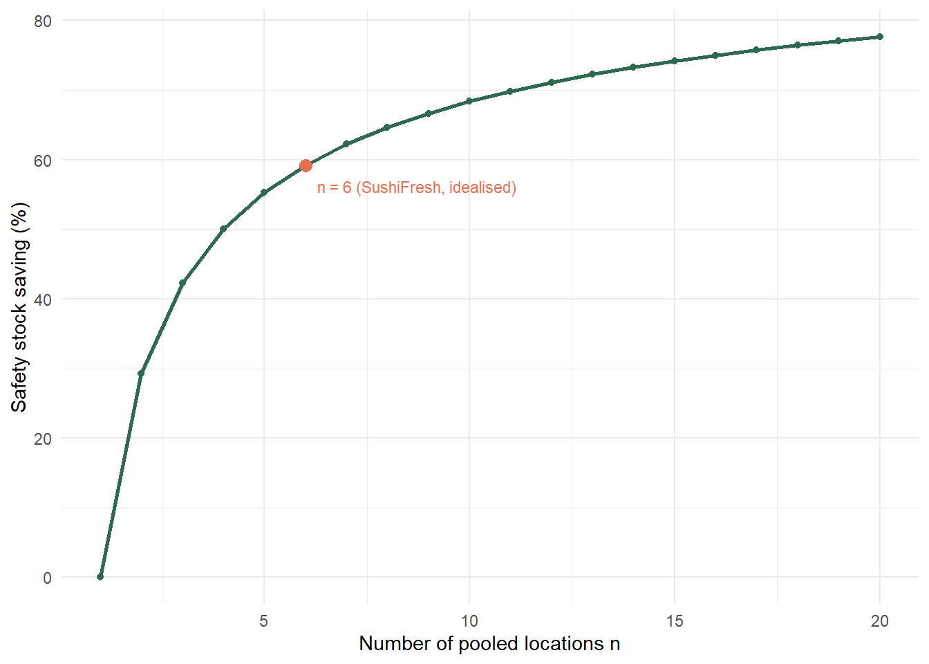
Both implementations deliver identical results: with six idealised **identical** locations with $\sigma = 29.33$ and $\alpha = 95\,\%$, the saving is around 59.2% — noticeably more than the 56.0% calculated for the actual, heterogeneous SushiFresh stores (see previous section). As $n$ increases, the relative saving in the idealised case continues to grow, but at a **diminishing marginal rate** — the jump from $n=1$ to $n=4$ brings more additional saving than the jump from $n=16$ to $n=20$:
```{r}
#| label: ch6-sqrt-law-plot
#| fig-cap: "Relative saving in safety stock as a function of the number of locations n (idealised, sigma = 29.33)"
n_seq <- 1:20

einsparung_df <- tibble(n = n_seq) |>
  mutate(einsparung = map_dbl(n, ~ pooling_safety_stock(.x, sigma = sigma_mean, z = qnorm(0.95))$savings_pct))

ggplot(einsparung_df, aes(x = n, y = einsparung)) +
  geom_line(color = "#2D6A4F", linewidth = 1) +
  geom_point(color = "#2D6A4F") +
  geom_point(data = filter(einsparung_df, n == 6), color = "#E76F51", size = 3) +
  annotate("text", x = 6.3, y = einsparung_df$einsparung[6] - 3,
           label = "n = 6 (SushiFresh, idealised)", hjust = 0, size = 3, color = "#E76F51") +
  labs(x = "Number of pooled locations n", y = "Safety stock saving (%)") +
  theme_minimal()
```
This diminishing marginal benefit is the economic reason why, in practice, companies rarely fully centralise an arbitrary number of warehouse locations: the first few merged locations deliver the greatest effect, whereas further centralisation brings only small additional savings while transport and coordination costs rise at the same time (analogous to the chaining argument above). Moreover, the square-root law in this simple form holds only under the assumption of **independent** demand ($\rho=0$) and **identical** locations — with positively correlated or differently sized locations, the saving is correspondingly smaller, as shown in the previous sections.
## Limits of the Normality Assumption: A Simulated Daily Demand Time Series
The examples so far were based on the assumption of (near-)normally distributed demand or on small, manageable data sets. Real sales data are rarely so well behaved: public holidays, special promotions or sudden changes in the weather occasionally generate **demand peaks** that violate a simple normality assumption. To conclude this chapter, this effect is examined using a **simulated** daily demand time series for the Frankfurt and Offenbach stores — deliberately generated synthetically (reproducible with `set.seed()`), but with occasional, shared "holiday peaks" that replicate typical properties of real sales data:
```{r}
#| label: ch6-simulierte-realistische-daten
#| message: false
set.seed(616)
n_tage <- 250

# Base daily demand: normally distributed around the known store parameters,
# but with somewhat lower "base dispersion", because the peak days are
# added separately
frankfurt <- pmax(30, round(rnorm(n_tage, mean = 280, sd = 55 * 0.7)))
offenbach <- pmax(10, round(rnorm(n_tage, mean = 95,  sd = 22 * 0.7)))

# Common demand drivers: on 6 random days (public holidays, events)
# BOTH stores spike considerably more strongly at the same time
spitzentage <- sample(seq_len(n_tage), size = 6)
frankfurt[spitzentage] <- frankfurt[spitzentage] + round(runif(6, 220, 420))
offenbach[spitzentage] <- offenbach[spitzentage] + round(runif(6, 70, 150))

sim_df <- tibble(tag = seq_len(n_tage), Frankfurt = frankfurt, Offenbach = offenbach,
                  Pool = frankfurt + offenbach)

sim_df |>
  summarise(mu_Frankfurt = mean(Frankfurt), sig_Frankfurt = sd(Frankfurt),
            mu_Offenbach = mean(Offenbach), sig_Offenbach = sd(Offenbach),
            rho = cor(Frankfurt, Offenbach))
```
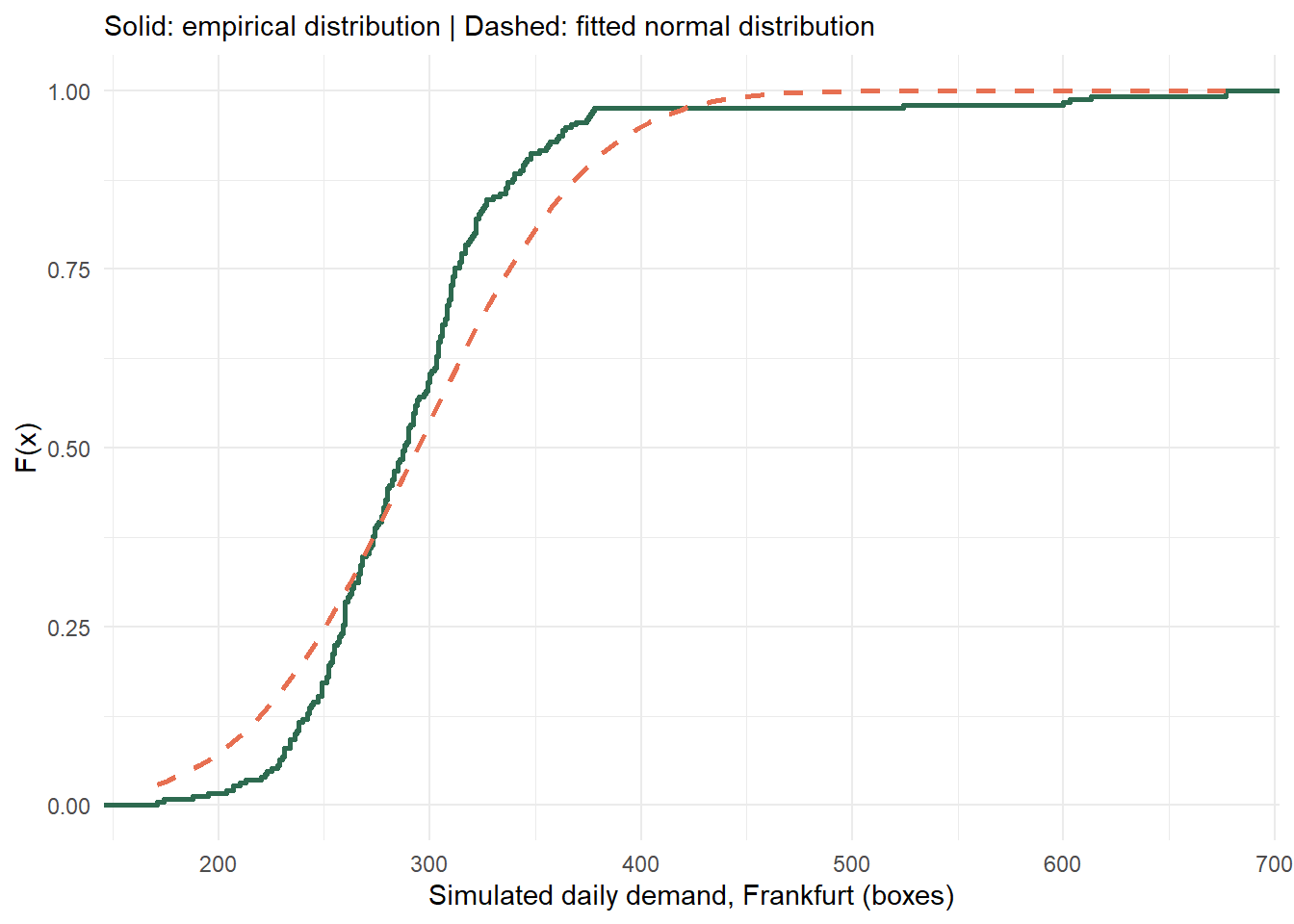
What stands out are the isolated **extreme peaks** on the simulated public holidays — they drive the standard deviation of both series above the level of the "normal" days and raise the question of whether the normality assumption from the previous section is still admissible here at all:
```{r}
#| label: ch6-real-ecdf-vs-normal
#| fig-cap: "ECDF vs. fitted normal distribution: simulated daily demand in Frankfurt (holiday peaks dominate the fit)"
mu_f <- mean(frankfurt); sig_f <- sd(frankfurt)

ggplot(sim_df, aes(x = Frankfurt)) +
  stat_ecdf(geom = "step", color = "#2D6A4F", linewidth = 0.9) +
  stat_function(fun = pnorm, args = list(mean = mu_f, sd = sig_f),
                color = "#E76F51", linetype = "dashed", linewidth = 0.9) +
  labs(x = "Simulated daily demand, Frankfurt (boxes)", y = "F(x)",
       subtitle = "Solid: empirical distribution | Dashed: fitted normal distribution") +
  theme_minimal()
# Formal test for normality (Kolmogorov–Smirnov)
ks.test(frankfurt, "pnorm", mu_f, sig_f)$p.value
```
The extremely small p-value of the Kolmogorov–Smirnov test confirms the visual impression: because of the interspersed peak days, the simulated distribution is **clearly far from a normal distribution** — it is right-skewed with a long "peak demand" tail. Nevertheless, the pooling effect can be evaluated **empirically**, i.e. without any normality assumption at all, directly via `ecdf()` or `quantile()`:
```{r}
#| label: ch6-real-pooling-vergleich
#| tbl-cap: "Empirical vs. parametric safety stock for simulated store data affected by public holidays"
alpha_r <- 0.95
z_r <- qnorm(alpha_r)

# Empirical: quantiles directly from the simulated data
sb_f_emp  <- quantile(frankfurt, alpha_r, type = 1) - mu_f
sb_o_emp  <- quantile(offenbach, alpha_r, type = 1) - mean(offenbach)
sb_dez_emp <- sb_f_emp + sb_o_emp
sb_zen_emp <- quantile(sim_df$Pool, alpha_r, type = 1) - mean(sim_df$Pool)

# Parametric: apply the normality assumption despite the poor fit
sig_o <- sd(offenbach); rho_r <- cor(frankfurt, offenbach)
sb_dez_par <- z_r * (sig_f + sig_o)
sb_zen_par <- z_r * sqrt(sig_f^2 + sig_o^2 + 2 * rho_r * sig_f * sig_o)

tibble(
  Method = c("Empirical (ECDF)", "Parametric (normal distribution)"),
  SS_decentralised = round(c(sb_dez_emp, sb_dez_par), 1),
  SS_centralised   = round(c(sb_zen_emp, sb_zen_par), 1),
  Saving_percent = round(c((1 - sb_zen_emp / sb_dez_emp) * 100,
                                (1 - sb_zen_par / sb_dez_par) * 100), 1)
)
```
Two observations are instructive here. First: the shared holiday peaks generate a noticeable positive correlation between Frankfurt and Offenbach ($\hat\rho \approx$ `r round(cor(frankfurt, offenbach), 2)`) — nevertheless, pooling still yields a clearly positive saving here too, both empirically and parametrically, even if it is smaller than in the (uncorrelated) main result for all six stores. Second: **empirical and parametric safety stocks diverge considerably** — because of the peak-driven standard deviation, the parametric calculation delivers higher absolute values than the empirical quantile estimate. This is an important practical lesson: where the normality assumption fits the actual data poorly (which can easily be checked with an ECDF plot and `ks.test()`), the safety stock should be determined **empirically** rather than **parametrically** — otherwise individual extreme days lead to a massive over- or under-dimensioning of stock that is economically hard to justify. For the idealised, normally distributed main result of this chapter (289.5 vs. 127.5 boxes, see above), this simplification was deliberately accepted — for operational implementation in the central kitchen, however, as this example shows, a supplementary empirical check against actual sales data would be advisable.
## Summary
This chapter has shown that uncertainty in supply chains is not an avoidable planning failure, but a **structural consequence** of the temporal separation between the capacity decision (ex ante) and the realisation of demand (ex post). The implied uncertainty of a product — determined by demand uncertainty and supply variability — determines how responsive the corresponding supply chain should be designed to be; at SushiFresh, the short shelf life of the sushi boxes exacerbates this problem further. Safety stocks dampen this mismatch over time; their level follows directly from the desired $\alpha$ service level and the (empirical or parametric) demand distribution.
The unifying principle of the chapter was **pooling**: whether for production capacities (SushiFresh's pilot kitchens in Wiesbaden/Mainz, chaining) or for inventories (the six stores under decentralised and centralised supply) — bundling resources across several locations or periods enables **risk pooling** that improves service level and utilisation at the same time, without creating additional physical capacity. The **key result** of this chapter: consolidation onto a central kitchen reduces the required safety stock at $\alpha = 95\,\%$ from 289.5 boxes (decentralised, six stores individually) to 127.5 boxes (centralised, pooled) — a saving of 56.0%. Formally, this effect is captured by the **square-root law**: for independent, identical locations, safety stock grows only with $\sqrt{n}$ rather than linearly with $n$ — with diminishing marginal benefit as the number of locations increases. The fact that the actual saving (56.0%) lies somewhat below the idealised value for six identical locations (59.2%) also highlights an important limitation: a dominant, above-average volatile location such as Frankfurt reduces the relative pooling benefit. The benefit of pooling furthermore depends crucially on the **correlation** between the pooled demands: it is greatest with negative correlation, falls noticeably for positively correlated (e.g. geographically neighbouring) locations and disappears completely with perfect positive correlation.
On the R side, this chapter introduced the tools for **modelling uncertainty**: the function family `rnorm()`/`dnorm()`/`pnorm()`/`qnorm()` for the normal distribution, `set.seed()` for the reproducibility of random experiments, `replicate()` and `MASS::mvrnorm()` for Monte Carlo simulations with correlated random variables, and `ecdf()` and `quantile()` for the data-driven, distribution-free evaluation of empirical observations. These tools are not limited to pooling — they form the basis for the **newsvendor model** in @sec-newsvendor, where (again using the example of the Frankfurt store) the focus is on determining an optimal order quantity under uncertainty.
::: {.kontrollfragen}
**Review questions**
1. What distinguishes the *implied uncertainty* of a product from its pure demand uncertainty? Place SushiFresh's sushi boxes on the *implied uncertainty spectrum* and justify your classification.
2. Why, with fixed capacity and stochastic demand, can over- and under-utilisation occur simultaneously at different locations in the same period?
3. Explain the difference between one-sided and two-sided capacity pooling using the example of the two SushiFresh pilot kitchens in Wiesbaden and Mainz. Why does pooling improve all service metrics simultaneously without creating additional capacity?
4. What is meant by *chaining*, and why does a chain structure with only $2n$ instead of $n^2$ links already achieve a large part of the full pooling benefit?
5. Define the $\alpha$ service level formally. How can the corresponding safety stock be determined from historical data without making a distributional assumption?
6. Derive the formula for the central safety stock of two pooled, normally distributed locations. For which value of the correlation $\rho$ does the pooling benefit disappear completely, and why?
7. Calculate the decentralised and the centralised safety stock for the six SushiFresh stores at $\alpha = 95\,\%$. Why is the actual saving (56.0%) lower than the saving that would result for six *identical* locations with the same average dispersion (59.2%)?
8. In which situations should safety stock be determined empirically rather than parametrically (via the normal distribution)? Use the results of the simulated Frankfurt/Offenbach case example in your answer.
:::