# Facility Location Planning I – Qualitative and Continuous Methods {#sec-standort-1}
::: {.lernziele}
**Learning objectives**
- **Classify** location decisions within strategic supply chain design and **distinguish** them from operational decisions,
- systematically **capture and evaluate** qualitative location factors,
- **explain** the scoring model (utility analysis) and the Analytic Hierarchy Process (AHP) **and apply them to a case example**,
- **explain** the properties of different distance metrics (Euclidean, Manhattan, geographic) and **compute** them in R,
- **derive, programme and interpret** the centre-of-gravity method and the Weiszfeld algorithm yourself,
- **apply** basic R control structures (loops, matrices, `apply` functions, custom functions with a stopping criterion).
:::
```{r}
#| label: ch4-setup
#| echo: false
#| warning: false
#| message: false
# Load helper functions from R/scm_functions.R (incl. center_of_gravity(),
# weiszfeld(), haversine(), ahp_priority_vector(), ahp_consistency())
source("../R/scm_functions.R")
library(tidyverse)
library(knitr)
library(kableExtra)
```
## Location decisions in strategic supply chain design
Chapter [-@sec-logistikkosten] showed that supply chain decisions are guided by a system of objectives that mediates between costs, service level and other target variables, and that logistics costs depend to a considerable extent on the spatial structure of a network. This chapter starts precisely from that spatial structure: the question is **where** a company should locate its plants, warehouses, transshipment points or sales outlets so that the network as a whole resolves the trade-off between cost and service as well as possible.
Location decisions belong to **strategic network planning** and differ fundamentally in several respects from operational decisions such as order quantity planning, which is covered in later chapters. First, they are as a rule **capital-intensive and binding in the long term**: a plant or a central warehouse cannot easily be relocated when demand patterns change. Second, the decision space is **multidimensional** – besides transport and construction costs, the labour market, infrastructure, taxes, political stability or proximity to customers play a role, and these criteria cannot always be expressed in a common unit (e.g. euros). Third, much of the relevant information is **uncertain or has to be assessed subjectively**, such as the future development of a regional labour market or “location quality” in the soft sense. These three properties – irreversibility, multidimensionality and uncertainty – explain why facility location planning has developed its own range of methods that goes well beyond a simple cost comparison [@kik2022standortplanung].
The facility location planning process typically runs through several phases with a decreasing level of aggregation: at a first, global level, continents or countries are pre-selected on the basis of a few highly aggregated factors (e.g. market access, wage level, political risk). At a second, regional level, the search space is narrowed down to economic areas or regions, where the requirements can already be formulated much more precisely. Only at a third, local level is a concrete site determined – a plot of land, a municipality, a junction in the transport network [@chopra2025supply].
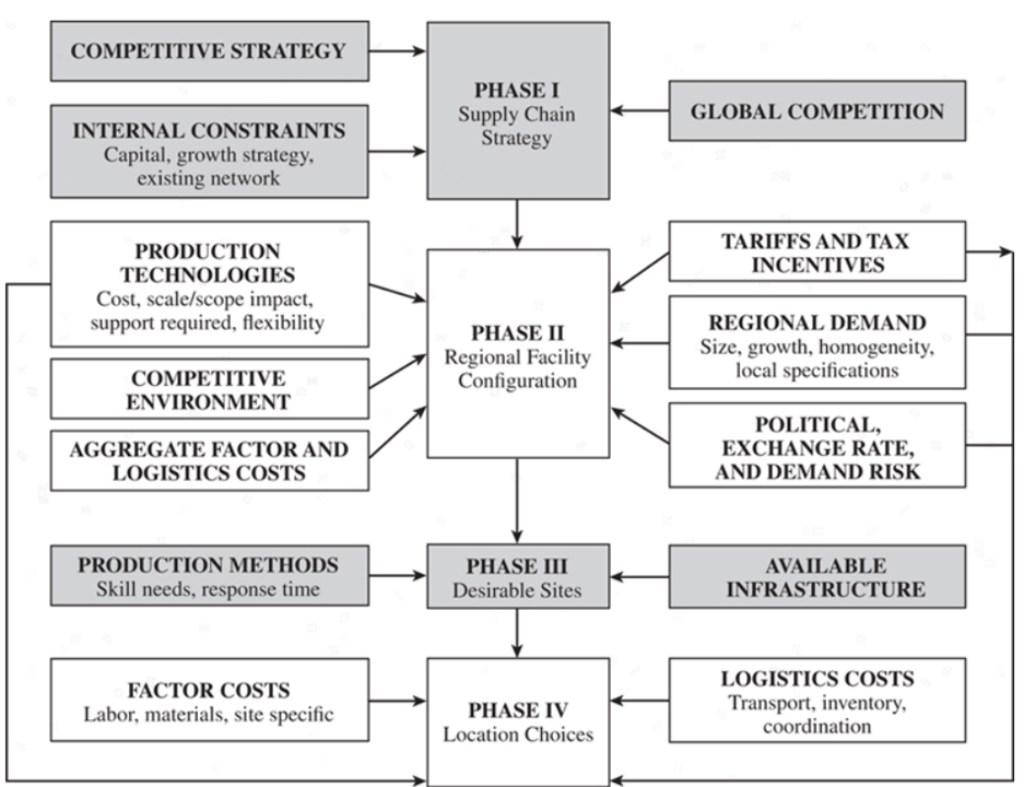{#fig-phasen-standortwahl width="85%"}
::: {.vertiefung}
**In depth (theory): The Supply Chain Planning Matrix**
The lecture places facility location planning within the **Supply Chain Planning Matrix** [@stadtler2000supply]. The matrix spans two dimensions: horizontally the value creation processes (procurement, production, distribution, sales), vertically the planning horizon (long, medium and short term). Each cell contains typical planning tasks — such as materials programme and supplier selection (long term, procurement), master production scheduling (medium term, production) or vehicle routing (short term, distribution). The long-term row across all processes is called **strategic network planning**: it determines which sites exist, what capacity they have and which transport links connect them.
Two properties of this matrix are important for understanding the following chapters. First, decisions act **top-down**: strategic network planning sets the framework within which medium-term quantity planning and short-term scheduling take place. A poorly located warehouse cannot be compensated for by even the best vehicle routing. Second, there is **bottom-up feedback**: in order to evaluate sites sensibly, the later operational costs (transport, inventory) must be anticipated at least approximately. Location models therefore work with aggregated quantities — average daily demand, transport cost rates per kilometre — that represent the operational level in simplified form. Chapters [-@sec-unsicherheit-pooling] to [-@sec-bullwhip] will later show which additional effects (inventory, uncertainty, bullwhip) are not yet visible at this simplified level.
:::
The slides also highlight why evaluating sites is so difficult: location decisions are **irreversible in the short term** and create **path dependencies** (later decisions build on the network once chosen), they are **multidimensional** (their effects on the system of objectives from Chapter [-@sec-logistikkosten] are hard to oversee) and they are **subjective** (the assessment of soft factors varies between decision-makers, and their importance is weighted differently).
Correspondingly broad is the range of **facility location planning methods** [@kik2022standortplanung]. *Qualitative methods* are heuristic, mostly survey-based methods that bring together an overall picture of opinion and individual assessments. Among the *quantitative methods*, **optimisation** requires a clearly delimited decision space (the options) and a one-dimensional system of objectives (e.g. costs); **simulation** can represent complex, multidimensional cause-and-effect relationships but is laborious and hard to transfer; **game-theoretic** approaches anticipate the behaviour of competitors, for example to maximise the sales of a retail site; and **investment appraisal** evaluates sites solely on the basis of monetary quantities over their useful life. This chapter and the next cover qualitative methods and optimisation models, because these two are most frequently combined in practice.
For the actual evaluation of sites (or location regions), two classes of methods are available in principle. **Qualitative methods** are heuristic, often survey-based evaluation approaches that combine an overall picture from several, usually also soft, criteria; they are particularly suitable for pre-selection among a limited number of discrete alternatives. **Quantitative methods**, by contrast, formulate the location search as an optimisation problem with an explicit objective function. In this chapter, we cover the **scoring model (utility analysis)** and the **Analytic Hierarchy Process (AHP)** from the qualitative family; we then turn to **continuous** quantitative methods, in which the site is not selected from a given list but determined as an arbitrary point in a plane. The **discrete** quantitative methods, in which a cost-minimal subset has to be selected from a finite set of potential sites, follow in Chapter [-@sec-standort-2].
Which location factors are relevant at all depends heavily on the individual case. Roughly, they can be divided into **hard** factors (transport costs, wages, taxes, land prices – directly measurable in monetary terms) and **soft** factors (quality of life, image of the region, availability of skilled labour, political stability). Soft factors defy direct cost accounting but influence location quality just as strongly – and qualitative evaluation methods are designed precisely for capturing them systematically.
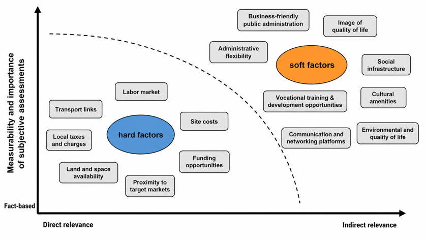{#fig-standortfaktoren width="80%"}
### The case study of this chapter: SushiFresh GmbH
We apply all methods in this chapter consistently to one and the same continuous case example, which will also accompany us in the following chapters on network and inventory planning: **SushiFresh GmbH**, a fictitious regional producer of fresh sushi boxes in the Rhine-Main area. SushiFresh supplies six supermarket stores every day with differing but largely known demand:
```{r}
#| label: ch4-sushifresh-filialen
#| echo: true
# Six supplied stores with coordinates (WGS84), mean daily demand
# mu (in sushi boxes) and its standard deviation sigma
filialen <- tibble(
  Filiale = c("Wiesbaden", "Mainz", "Frankfurt", "Ruesselsheim", "Darmstadt", "Offenbach"),
  lat   = c(50.0782, 50.0000, 50.1109, 49.9904, 49.8728, 50.0956),
  lon   = c(8.2398,  8.2711,  8.6821,  8.4116,  8.6512,  8.7761),
  mu    = c(120, 150, 280, 90, 110, 95),
  sigma = c(25, 30, 55, 20, 24, 22)
)
filialen |> rename(Store = Filiale)   # English column name for display
```
In addition to the existing deliveries, management is considering building its own production facility in the Rhine-Main area and has identified three commercial plots as candidate sites:
```{r}
#| label: ch4-sushifresh-standorte
#| echo: true
# Three candidate sites for the new production facility
standorte <- tibble(
  Standort = c("Wiesbaden-Erbenheim", "Mainz-Hechtsheim", "Raunheim"),
  lat = c(50.0632, 49.9698, 50.0000),
  lon = c(8.2999,  8.2831,  8.4650),
  Fixkosten = c(180000, 210000, 260000)
)
standorte |> rename(Site = Standort, `Fixed costs` = Fixkosten)   # English column names for display
# Transport cost rate per box and kilometre (needed again later)
transportkostensatz <- 0.02
```
Wiesbaden-Erbenheim is a business park with direct access to the A66/A3 and comparatively low land prices; Mainz-Hechtsheim is located on the A60/A63 and close to the Rhine, which favours the delivery of fish, but is more expensive; finally, Raunheim lies close to Frankfurt Airport with very good connections to the A3/A5 but charges the highest commercial rents. The column `Fixkosten` contains the one-off investment and development costs of the plots (fit-out, refrigeration technology, production equipment); in Chapter [-@sec-standort-2] they are spread over a useful life of five years and thus converted into annual fixed costs. Together, the six stores demand `r sum(filialen$mu)` sushi boxes per day; with 280 boxes, Frankfurt is by far the largest store – we will meet it again in Chapter [-@sec-newsvendor] as an example for the newsvendor formula. This chapter first addresses how SushiFresh can systematically evaluate the three candidate sites and how the company – independently of the three given plots – can determine, purely by calculation, the point in the sales area that minimises transport costs.
## Qualitative location evaluation
### The scoring model (utility analysis)
::: {.definition}
**Definition: Scoring model (utility analysis)**
The **scoring model (utility analysis, German *Nutzwertanalyse*, NWA)** is an additive multi-criteria evaluation method. For each alternative $j$, an **overall utility value** $N_j$ is formed across all criteria $k=1,\dots,K$ as the weighted sum of the partial utility values $w_{jk}$:
$$
N_j = \sum_{k=1}^{K} g_k \cdot w_{jk}, \qquad \sum_{k=1}^{K} g_k = 1,
$$
where $g_k$ is the weight of criterion $k$ and $w_{jk}$ is the rating of alternative $j$ with respect to criterion $k$ (usually awarded on a points scale, e.g. 0–10).
:::
The scoring model follows a clearly structured, five-step procedure: first, the relevant evaluation criteria are defined, then their weights are determined (e.g. by expert estimation or pairwise comparison). Next, the alternatives are rated for each criterion, the weighted partial utility values are aggregated into the overall utility value, and finally the alternatives are ranked according to this overall utility value.
This additive structure makes the scoring model simple to apply and easy to follow – but it also harbours a methodological weakness that is best illustrated with a numerical example.
::: callout-note
## Case example: Production site for SushiFresh
SushiFresh management evaluates the three candidate sites Wiesbaden-Erbenheim, Mainz-Hechtsheim and Raunheim on the basis of three criteria – weighted equally here for simplicity: **transport proximity** to the six stores, **rental costs** and **availability of skilled labour**. Wiesbaden-Erbenheim is strongest on rental costs (lowest fixed costs), Raunheim on transport proximity to the store network, while Mainz-Hechtsheim leads on the availability of skilled labour – it offers good access to training institutions in catering and food technology.
:::
```{r}
#| label: ch4-nwa-tabelle
#| echo: true
# Raw data of the case study: three criteria, equally weighted (1/3 per criterion),
# ratings of the three candidate sites on a scale from 0 (poor) to 10 (good)
nwa <- tibble(
  Kriterium = c(
    "Transport proximity",
    "Rental costs",
    "Skilled labour availability"
  ),
  Gewicht = c(1/3, 1/3, 1/3),
  `WI-Erbenheim`  = c(5, 8, 2),
  `MZ-Hechtsheim` = c(2, 5, 8),
  Raunheim        = c(8, 2, 5)
)

# Overall utility value per site: sum of weight * rating across all criteria
nutzwert <- c(
  `WI-Erbenheim`  = sum(nwa$Gewicht * nwa$`WI-Erbenheim`),
  `MZ-Hechtsheim` = sum(nwa$Gewicht * nwa$`MZ-Hechtsheim`),
  Raunheim        = sum(nwa$Gewicht * nwa$Raunheim)
)
nutzwert
```
```{r}
#| label: ch4-nwa-kable
#| echo: false
nwa_tab <- bind_rows(
nwa,
tibble(Kriterium = "Utility value", Gewicht = NA,
`WI-Erbenheim` = nutzwert["WI-Erbenheim"],
`MZ-Hechtsheim` = nutzwert["MZ-Hechtsheim"],
Raunheim = nutzwert["Raunheim"])
)
nwa_tab |>
mutate(
Gewicht = ifelse(is.na(Gewicht), "", sprintf("%.2f", Gewicht)),
across(c(`WI-Erbenheim`, `MZ-Hechtsheim`, Raunheim), ~ sprintf("%.1f", .x))
) |>
kable(col.names = c("Criterion", "Weight", "WI-Erbenheim", "MZ-Hechtsheim", "Raunheim"),
align = "lccc") |>
kable_styling(full_width = FALSE)
```
At first glance, the result is surprising: **all three sites achieve exactly the same overall utility value of `r sprintf("%.1f", nutzwert[1])`** – even though their strength–weakness profiles are completely different: Wiesbaden-Erbenheim scores on rental costs but loses on the availability of skilled labour; Mainz-Hechtsheim scores on skilled labour but loses on transport proximity; Raunheim scores on transport proximity but loses on rental costs. The reason for the identical result lies in the additive aggregation: a weak rating on one criterion can be **compensated** by a correspondingly strong rating on another criterion. This **compensability** is the central methodological weakness of the scoring model. It raises several follow-on problems:
- The additive model can only be interpreted to a limited extent, because it implicitly assumes that the criteria are **utility-independent** – i.e. that the utility contribution of one criterion does not change depending on how well or badly other criteria turn out. In practice, this assumption is often questionable.
- The results are sensitive to the chosen weighting; small shifts in the weights $g_k$ can reverse the ranking of the alternatives.
- There is a risk of **objective splitting**: an objective that is actually coherent is broken down into many individual criteria whose weights can hardly be set in a comprehensible way.
These weaknesses motivate a method that derives the criteria and alternative weights more systematically – via **pairwise comparisons** instead of directly estimated scores: the Analytic Hierarchy Process.
### The Analytic Hierarchy Process (AHP)
::: {.definition}
**Definition: Analytic Hierarchy Process**
The **Analytic Hierarchy Process (AHP)** is a multi-level multi-criteria decision method that derives priorities – for criteria as well as for alternatives – from **pairwise comparisons**. Instead of estimating scores directly, the decision-maker assesses two elements against each other at a time (“How much more important is A than B?”) on a defined scale. From the resulting **pairwise comparison matrix**, a priority vector is then derived that can be interpreted as a ranking or weighting.
:::
The AHP proceeds in five steps: (1) form pairwise comparisons between all alternatives for each evaluation criterion, (2) derive a ranking of the alternatives for each criterion from these (“synthesis”), (3) form pairwise comparisons between all evaluation criteria, (4) derive a ranking of the criteria from these, and (5) combine both rankings into an overall score per alternative.
The steps follow a **bottom-up hierarchy** (@fig-ahp-hierarchy): first, the contribution of each alternative to each criterion is assessed; then the contribution of each criterion to the overall objective; finally, both are combined to identify the best alternative.
::: {#fig-ahp-hierarchy}
::: {.ahp-hierarchy}
::: {.ahp-level}
**Bottom level:** Determine how the alternatives contribute to the criteria.
:::
::: {.ahp-arrow}
⇓
:::
::: {.ahp-level}
**Medium level:** Determine how the evaluation criteria contribute to achieving the objective.
:::
::: {.ahp-arrow}
⇓
:::
::: {.ahp-level}
**Top level:** Determine the best of the given alternatives (objective).
:::
:::
Bottom-up hierarchy of the AHP [after @klein2011planung, p. 361]
:::
Pairwise comparisons are usually recorded on a nine-point scale ranging from “equally important” (value 1) to “extremely preferred” (value 9); the reciprocal values $1/9$ to $1$ express the opposite direction of preference. A pairwise comparison matrix $A$ with entries $a_{ij}$ (“how much more important is $i$ than $j$?”) is therefore **reciprocal**: $a_{ji} = 1/a_{ij}$, and the diagonal always contains ones. From a perfectly consistent matrix, the priority vector could be read directly from a single row or column; in practice, however, expert assessments are never perfectly consistent, which is why the priority vector is determined by averaging – computationally via the **dominant eigenvector** of the matrix, approximated e.g. by the geometric mean of the rows.
::: callout-note
## Case example: AHP for the SushiFresh production site
Instead of estimating scores directly, SushiFresh management now compares the three candidate sites Wiesbaden-Erbenheim, Mainz-Hechtsheim and Raunheim pairwise – both against each other for each criterion and the three criteria **transport proximity**, **rental costs** and **availability of skilled labour** against one another.
:::
To represent the three pairwise comparison matrices (one per criterion) and the criteria comparison matrix in R, we need a data structure that – unlike a `data.frame` – is **rectangular and purely numeric** from the outset and can be processed using the rules of linear algebra (matrix multiplication, transposition): the **matrix**.
::: {.r-exkurs}
**R aside: Matrices in R**
A matrix is created with `matrix()`. The vector of values is arranged row-wise or column-wise into the desired shape; `byrow = TRUE` ensures that the values are filled in row by row (instead of R's default column-wise order). Row and column names can be assigned with `dimnames`. Individual elements, entire rows or columns are accessed via square brackets with two indices `[row, column]` – an empty index stands for “all”:
```{r}
#| label: ch4-matrix-exkurs
#| echo: true
# Create a 3x3 matrix with row and column names: pairwise comparison
# of the three candidate sites with respect to the criterion transport proximity
m <- matrix(
  c(1,   2,   1/2,
    1/2, 1,   1/3,
    2,   3,   1),
  nrow = 3, byrow = TRUE,
  dimnames = list(c("WI-Erb", "MZ-Hech", "Raunheim"), c("WI-Erb", "MZ-Hech", "Raunheim"))
)
m
# Single element: row 1, column 2 -> "How strongly is WI-Erb preferred over MZ-Hech?"
m[1, 2]
# Entire 2nd row: comparison of MZ-Hech with all three sites
m[2, ]
# Dimensions of the matrix (rows, columns)
dim(m)
```
For two matrices `X` (dimension $m \times n$) and `Y` (dimension $n \times p$), the operator `%*%` computes the **matrix product** $X\,Y$ (dimension $m \times p$) in the sense of linear algebra – unlike `X * Y`, which only multiplies element-wise. We use `%*%` twice below: once to combine a distance matrix with a demand vector, and once to combine the criteria weights with the ratings of the alternatives into an overall AHP score.
:::
This allows the three pairwise comparison matrices from the case example to be reproduced directly in R:
```{r}
#| label: ch4-ahp-matrizen
#| echo: true
# Pairwise comparisons of the three candidate sites per criterion (Saaty scale 1-9 or reciprocals)
transportnaehe <- matrix(
  c(1,   2,   1/2,
    1/2, 1,   1/3,
    2,   3,   1),
  nrow = 3, byrow = TRUE,
  dimnames = list(c("WI-Erb", "MZ-Hech", "Raunheim"), c("WI-Erb", "MZ-Hech", "Raunheim"))
)

mietkosten <- matrix(
  c(1,   2,   4,
    1/2, 1,   2,
    1/4, 1/2, 1),
  nrow = 3, byrow = TRUE,
  dimnames = list(c("WI-Erb", "MZ-Hech", "Raunheim"), c("WI-Erb", "MZ-Hech", "Raunheim"))
)

fachkraefte <- matrix(
  c(1,   1/7, 2,
    7,   1,   5,
    1/2, 1/5, 1),
  nrow = 3, byrow = TRUE,
  dimnames = list(c("WI-Erb", "MZ-Hech", "Raunheim"), c("WI-Erb", "MZ-Hech", "Raunheim"))
)
```
The matrix `mietkosten` (rental costs) directly reflects the fixed costs of the three plots (€180,000 / €210,000 / €260,000): Wiesbaden-Erbenheim is clearly preferred over Raunheim with a value of 4. For each of these three matrices, `ahp_priority_vector()` from `R/scm_functions.R` returns the corresponding priority vector (the relative site preferences per criterion). Instead of calling the function three times individually, we bundle the three matrices in a **list** and apply the function to each list element with `sapply()`.
::: {.r-exkurs}
**R aside: `sapply()` and `apply()`**
`sapply(X, FUN)` applies a function `FUN` to each element of `X` and simplifies the result to a vector or matrix where possible. If `X` – as here – is a **list of matrices** and `FUN` returns a vector of the same length for each element, the result is a matrix in which each column corresponds to one list element. `sapply()` thus saves writing a loop by hand when the same function is to be applied repeatedly to several objects.
Closely related is `apply(X, MARGIN, FUN)`, which applies a function row-wise (`MARGIN = 1`) or column-wise (`MARGIN = 2`) to a **single** matrix. Internally, `ahp_priority_vector()` uses exactly this pattern to compute the geometric mean for each row of a pairwise comparison matrix – a common, numerically stable approximation of the actually exact eigenvector method.
```{r}
#| label: ch4-ahp-sapply
#| echo: true
# List of all three criteria matrices
kriterien_matrizen <- list(
  Transport      = transportnaehe,
  Rent           = mietkosten,
  Skilled_labour = fachkraefte
)

# sapply() applies ahp_priority_vector() to each matrix in the list and
# returns the three preference vectors as a joint matrix (sites x criteria)
praeferenz_matrix <- sapply(kriterien_matrizen, ahp_priority_vector)
praeferenz_matrix
```
:::
The table `praeferenz_matrix` shows: Raunheim clearly dominates on transport proximity (approx. 54%), Wiesbaden-Erbenheim on rental costs (approx. 57%), and Mainz-Hechtsheim very clearly on the availability of skilled labour (approx. 74%) – so, as in the scoring model, each of the three sites plays to a different strength. This completes step 2 of the AHP (synthesis per criterion); what is still missing is the ranking of the three criteria themselves (steps 3 and 4), which again requires a pairwise comparison matrix – this time between the criteria rather than between the sites.
```{r}
#| label: ch4-ahp-kriterien
#| echo: true
# Pairwise comparison of the three evaluation criteria with one another
kriterien_vergleich <- matrix(
  c(1,   3,   2,
    1/3, 1,   1/5,
    1/2, 5,   1),
  nrow = 3, byrow = TRUE,
  dimnames = list(
    c("Transport", "Rent", "Skilled_labour"),
    c("Transport", "Rent", "Skilled_labour")
  )
)

kriterien_gewichte <- ahp_priority_vector(kriterien_vergleich)
kriterien_gewichte
```
With around `r sprintf("%.0f", kriterien_gewichte["Transport"]*100)`%, transport proximity receives by far the highest weight, followed by availability of skilled labour (approx. `r sprintf("%.0f", kriterien_gewichte["Skilled_labour"]*100)`%); with around `r sprintf("%.0f", kriterien_gewichte["Rent"]*100)`%, rental costs play a comparatively minor role. Before we use these weights further, we check whether the underlying pairwise comparison matrix is **consistent** enough at all to allow robust conclusions. Consistency here means **transitivity of intensities**: anyone who considers transport proximity three times as important as rental costs ($a_{TM}=3$) and skilled labour five times as important as rental costs ($a_{FM}=5$) should logically consider transport proximity only $3/5 = 0.6$ times as important as skilled labour. In fact, however, $a_{TF}=2$ was stated – i.e. transport proximity twice as important as skilled labour. A perfectly consistent matrix satisfies $a_{ik} = a_{ij}\cdot a_{jk}$ for all $i,j,k$; the more strongly this condition is violated, the larger the largest eigenvalue of the matrix becomes relative to $n$. Formally, the **consistency index**
$$
CI = \frac{\bar{\lambda} - n}{n - 1}
$$
is computed for this purpose, where $n$ is the number of criteria and $\bar{\lambda}$ is the (approximated) largest eigenvalue of the matrix, obtained by dividing the product of the matrix and the priority vector component-wise by the priority vector and taking the average. Relative to a randomly generated **random index** $RI$ (tabulated by Saaty as a function of $n$), this yields the **consistency ratio**
$$
CR = \frac{CI}{RI}.
$$
As a rule of thumb, a matrix is considered sufficiently consistent if $CR < 0.10$; for larger values, the pairwise comparisons should be revised.
```{r}
#| label: ch4-ahp-konsistenz
#| echo: true
konsistenz <- ahp_consistency(kriterien_vergleich, kriterien_gewichte)
konsistenz
```
With $CI \approx `r sprintf("%.3f", konsistenz$CI)`$ and $CR \approx `r sprintf("%.2f", konsistenz$CR)`$, the criteria matrix lies **above** the 10% threshold. The intransitivity between transport proximity, skilled labour and rental costs described above is therefore too large for the weights to be adopted unchecked. In practice, one would ask the decision-makers to reconsider their comparisons – for instance, correcting the comparison of transport proximity versus skilled labour from 2 to 1/2, which would make the matrix almost consistent. For the teaching example, we continue calculating with the original judgements from the lecture but keep this caveat in mind: it shows precisely the benefit of the AHP, which – unlike the scoring model – makes inconsistencies visible in the first place.
::: {.callout-note}
## Note on the lecture slides
On the slides, the consistency value $CI = (\bar{P}-n)/(n-1) \approx 0.08$ is calculated. This value is the **consistency index** $CI$. For the verdict “consistent/inconsistent”, it still has to be divided by the random index $RI = 0.58$ (for $n=3$); only the resulting consistency ratio $CR \approx 0.14$ is compared with the 10% threshold.
:::
In the last step, the site–criteria matrix and the criteria weight vector are combined into an **overall score per site** using the matrix product `%*%` – exactly the operation announced in the R aside on matrices:
```{r}
#| label: ch4-ahp-scores
#| echo: true
scores <- praeferenz_matrix %*% kriterien_gewichte
scores
```
**Mainz-Hechtsheim** achieves the highest value with a score of around `r sprintf("%.3f", scores["MZ-Hech", 1])`, ahead of Raunheim (`r sprintf("%.3f", scores["Raunheim", 1])`) and Wiesbaden-Erbenheim (`r sprintf("%.3f", scores["WI-Erb", 1])`). At first glance, the result is surprising, since by far the highest criterion weight belongs to transport proximity, where Raunheim clearly leads. The decisive factor is the **strength** of the preference on skilled labour: there, Mainz-Hechtsheim is rated as “strongly preferred” (7) over Wiesbaden-Erbenheim and receives around 74% of the criterion weight – with a criterion weight for skilled labour of around 38%, this is enough to more than make up for the deficit on transport proximity. The lead over Raunheim is narrow, however, and in view of the inconsistency found in the criteria matrix, a sensitivity analysis of the weights (see review questions) would be advisable before a final recommendation.
Compared with the scoring model, the AHP has two major advantages: first, pairwise comparison increases transparency, because decision-makers only have to weigh two elements against each other at a time instead of a complete ranking. Second, the AHP offers less scope for bias in individual assessments than the scoring model, because irrational or contradictory judgements can be explicitly uncovered via the consistency index – a diagnostic tool that the scoring model lacks and that actually triggers in the case example. Whether the qualitative recommendation in favour of Mainz-Hechtsheim is also confirmed by a purely quantitative cost analysis is deliberately left open at this point – we will return to it at the end of this chapter and then again in detail in Chapter [-@sec-standort-2].
::: {.vertiefung}
**In depth (theory): Why the eigenvector? – Computational approaches of the AHP**
The idea of the AHP [@saaty1980analytic] is best understood starting from the ideal case. Suppose the “true” weights of the alternatives are $w_1,\dots,w_n$ and the decision-maker judges without error. Then, as pairwise comparisons, they would state exactly the ratios $a_{ij} = w_i/w_j$. Multiplying such a matrix by the weight vector gives
$$
(A\,w)_i = \sum_{j=1}^n \frac{w_i}{w_j}\, w_j = n\, w_i \qquad\Longleftrightarrow\qquad A\,w = n\,w .
$$
The weight vector is therefore an **eigenvector** of the pairwise comparison matrix for the eigenvalue $n$. Because the matrix has rank 1 in this ideal case, all other eigenvalues are zero, and $n$ is the largest eigenvalue $\lambda_{\max}$. Real judgements are not perfectly consistent; then $\lambda_{\max} > n$, and Saaty proposes using the eigenvector belonging to the largest eigenvalue as the “best possible” weight vector. The deviation $\lambda_{\max} - n$ at the same time measures how strongly the judgements deviate from the consistent ideal case – from this, the consistency index $CI = (\lambda_{\max}-n)/(n-1)$ is derived. The random index $RI$ is the average $CI$ value of randomly filled reciprocal matrices of the same size; the consistency ratio $CR = CI/RI$ thus compares the observed inconsistency with that of a decision-maker “rolling dice”.
In practice, the eigenvector is often **approximated**. Two methods are common:
1. **Column normalisation and row mean** (the approach on the lecture slides): each column is divided by its column sum, and the average is then taken across each row. In the consistent case, each normalised column is already exactly the weight vector; in the case of inconsistency, averaging evens out the deviations.
2. **Geometric row mean** (used in `ahp_priority_vector()`): for each row, $\left(\prod_j a_{ij}\right)^{1/n}$ is formed and then normalised. This method also yields exactly $w$ in the consistent case and is moreover invariant to transposition (taking reciprocals) of the judgements.
For nearly consistent matrices, both methods and the exact eigenvector yield practically identical values; with stronger inconsistencies, they differ in the third decimal place. The following code reproduces the approach on the slides for the criteria matrix and compares it with the geometric mean and the exact eigenvector returned by `eigen()`:
```{r}
#| label: ch4-ahp-rechenwege
# 1) Column normalisation and row mean (approach on the slides)
spalten_normiert <- sweep(kriterien_vergleich, 2, colSums(kriterien_vergleich), "/")
w_spalten <- rowMeans(spalten_normiert)

# 2) Geometric row mean (ahp_priority_vector)
w_geo <- ahp_priority_vector(kriterien_vergleich)

# 3) Exact eigenvector for the largest eigenvalue
ev    <- eigen(kriterien_vergleich)
w_eig <- Re(ev$vectors[, 1]) / sum(Re(ev$vectors[, 1]))

round(cbind(`Column normalisation` = w_spalten, `Geometric mean` = w_geo, Eigenvector = w_eig), 3)
Re(ev$values[1]) # largest eigenvalue lambda_max (> n = 3 due to inconsistency)
```
:::
## Continuous facility location planning: the Steiner–Weber model
Both the scoring model and the AHP presuppose that a **manageable set of discrete alternatives** is already available to choose from – at SushiFresh, the three commercial plots actually available. Often, however, the location question arises differently: what is sought is not the best of several given addresses, but **the point in the plane** that minimises transport costs to a set of customer locations – at SushiFresh, the point in the Rhine-Main area that minimises the total distance to the six stores, regardless of whether a plot is available there at all. This question is addressed by **continuous facility location planning**, whose classic model goes back to Alfred Weber and is usually referred to in the literature as the **Steiner–Weber model** [@cooper1968locational; @thonemann2023operations].
The model makes four simplifying assumptions: there is a homogeneous plane (the sales area) containing a finite number of customer locations; for each customer location, a demand quantity is given that must be served in full; transport costs depend linearly on distance and quantity transported; and the time dimension is disregarded. Under these assumptions, the objective function is
$$
\min_{(x,y)}\; Z(x,y) = \sum_{i=1}^{n} a_i \cdot d\big((x,y),(u_i,v_i)\big),
$$
where $(x,y)$ are the sought coordinates of the new site, $(u_i, v_i)$ the coordinates of customer location $i$, $a_i$ its demand (at SushiFresh: boxes per day) and $d(\cdot)$ a **distance measure** still to be chosen.
The choice of $d(\cdot)$ is by no means secondary; it determines both the computational method and the result. For sites within a country or region in which transport routes run approximately “as the crow flies”, the **Euclidean distance** is suitable:
$$
d^{\text{eukl}}\big((x,y),(u_i,v_i)\big) = \sqrt{(x-u_i)^2 + (y-v_i)^2}.
$$
In city centres with a rectangular street grid or for in-plant transport along orthogonal aisles, the **Manhattan distance** (also rectilinear or $L_1$ distance) is often more realistic:
$$
d^{\text{man}}\big((x,y),(u_i,v_i)\big) = |x-u_i| + |y-v_i|.
$$
For actual network planning, in turn, **road distances** – the shortest paths in a real transport network – are the most accurate, but also the most laborious to compute, as they require a digital road network and a routing service. The following code shows by way of example how these three distance measures between the candidate site Wiesbaden-Erbenheim and the Frankfurt store can be computed with the packages `sf`, `osrm` and `leaflet` and compared on an interactive map. Since the road distance requires an online routing service (OSRM) and the retrieval of map tiles, the chunk is marked `eval: false` and is not executed during rendering.
```{r}
#| label: ch4-distanzen-karte
#| echo: true
#| eval: false
# Note: this chunk requires internet access (OpenStreetMap map tiles
# and the OSRM routing service for the road distance) and is therefore not
# executed when rendering the book (eval: false) - it only serves to
# illustrate how the three distance measures are compared in practice.

library(sf)
library(osrm)
library(leaflet)

standort_wi <- st_as_sf(data.frame(id = "Wiesbaden-Erbenheim", lon = 8.2999, lat = 50.0632),
                         coords = c("lon", "lat"), crs = 4326)
filiale_ffm <- st_as_sf(data.frame(id = "Frankfurt", lon = 8.6821, lat = 50.1109),
                         coords = c("lon", "lat"), crs = 4326)

# Shortest path in the real road network via the OSRM service
route <- osrmRoute(src = standort_wi, dst = filiale_ffm)

# Interactive map: road route in red, site/store as markers
leaflet() |>
  addProviderTiles(providers$OpenStreetMap.Mapnik) |>
  addPolylines(data = route, color = "red") |>
  addCircleMarkers(data = standort_wi, color = "black") |>
  addCircleMarkers(data = filiale_ffm, color = "purple")
```
In practice, the road distance between two points is almost always greater than the Euclidean and usually also greater than the Manhattan distance, since real road networks are neither straight nor strictly orthogonal. For the following derivations, we restrict ourselves – as the literature on the Steiner–Weber model predominantly does – to Euclidean and Manhattan distances, because closed-form or efficient iterative solution methods can be given for both [@daskin2013network; @drezner2002facility].
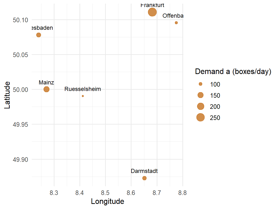
For the numerical examples in this section, we consistently use the SushiFresh data set with the six stores introduced above. Since the centre of gravity and the Weiszfeld algorithm were originally derived for **planar** (Cartesian) coordinates, we initially treat longitude and latitude here approximately as planar $x$/$y$ coordinates ($x = $ longitude, $y = $ latitude) – a deliberate didactic simplification whose limits we make explicitly visible at the end of this section using the haversine formula.
```{r}
#| label: ch4-filialen-plot
#| echo: true
#| fig-width: 6
#| fig-height: 4.5
#| fig-align: center
# Bubble chart: position = store, bubble size = demand
ggplot(filialen, aes(x = lon, y = lat)) +
  geom_point(aes(size = mu), color = "#c97a2b", alpha = 0.85) +
  geom_text(aes(label = Filiale), vjust = -1.2, size = 3.2) +
  labs(x = "Longitude", y = "Latitude", size = "Demand a (boxes/day)") +
  theme_minimal(base_size = 12)
```
### Centre of gravity: the quadratic approximation
The simplest approach to the Steiner–Weber problem is obtained if, in the objective function, one minimises not the (non-differentiable) Euclidean distance itself but its **square**:
$$
\min_{(x,y)}\; \tilde{Z}(x,y) = \sum_{i=1}^{n} a_i \left[(x-u_i)^2 + (y-v_i)^2\right].
$$
This objective function is separable in $x$ and $y$ and differentiable everywhere, so the minimum can be determined directly via the necessary optimality conditions. The partial derivative with respect to $x$ is
$$
\frac{\partial \tilde{Z}}{\partial x} = \sum_{i=1}^{n} 2\,a_i\,(x - u_i) \stackrel{!}{=} 0
\quad\Longleftrightarrow\quad
x \sum_{i=1}^{n} a_i = \sum_{i=1}^{n} a_i\, u_i,
$$
and analogously for $y$. Solving for $x$ and $y$ yields the **centre of gravity (CoG)**:
::: {.definition}
**Definition: Centre of gravity**
$$
x^{CoG} = \frac{\displaystyle\sum_{i=1}^{n} a_i\, u_i}{\displaystyle\sum_{i=1}^{n} a_i},
\qquad
y^{CoG} = \frac{\displaystyle\sum_{i=1}^{n} a_i\, v_i}{\displaystyle\sum_{i=1}^{n} a_i}.
$$
The centre of gravity is the **demand-weighted centroid** of all customer locations and minimises the sum of the weighted *squared* Euclidean distances.
:::
Since this derivation essentially consists of only three computational steps – calculating total demand, forming weighted coordinate sums, dividing – it can be reproduced in R directly and without any aids:
```{r}
#| label: ch4-cog-manual
#| echo: true
# Step 1: sum up total demand across all stores
gesamtnachfrage <- sum(filialen$mu)

# Step 2: form the demand-weighted sum of longitude and latitude
gewichtete_summe_lon <- sum(filialen$mu * filialen$lon)
gewichtete_summe_lat <- sum(filialen$mu * filialen$lat)

# Step 3: dividing by total demand yields the centroid
cog_lon <- gewichtete_summe_lon / gesamtnachfrage
cog_lat <- gewichtete_summe_lat / gesamtnachfrage

c(lon = cog_lon, lat = cog_lat)
```
As a check, the ready-made function `center_of_gravity()` from `R/scm_functions.R` – which encapsulates the same calculation but expects a `data.frame` with columns `x`, `y`, `demand` – returns the same result:
```{r}
#| label: ch4-cog-check
#| echo: true
center_of_gravity(data.frame(x = filialen$lon, y = filialen$lat, demand = filialen$mu))
```
The centre of gravity lies at $(x^{CoG}, y^{CoG}) \approx (`r sprintf("%.4f", cog_lon)`; `r sprintf("%.4f", cog_lat)`)$ – geographically roughly between Frankfurt and Rüsselsheim, well to the east of the three candidate sites. It is attractive because it can be computed in closed form **without iteration**. Strictly speaking, however, it does not solve the original Steiner–Weber problem, only its squared variant – and the two optima need not be identical. In particular, the CoG is more sensitive to distant outlier customers, because squared distances weight large distances disproportionately. For the *actual*, non-squared objective function, a different method is needed.
### The Weiszfeld algorithm: iterative solution of the true problem
To solve the original problem with linear (non-squared) Euclidean distances, we again form the necessary optimality condition, this time for
$$
Z(x,y) = \sum_{i=1}^{n} a_i \sqrt{(x-u_i)^2+(y-v_i)^2}.
$$
The partial derivative with respect to $x$ is
$$
\frac{\partial Z}{\partial x} = \sum_{i=1}^{n} a_i\, \frac{x - u_i}{d_i(x,y)} \stackrel{!}{=} 0,
\qquad d_i(x,y) = \sqrt{(x-u_i)^2+(y-v_i)^2}.
$$
Unlike with the squared objective function, $x$ here also appears in the denominator (via $d_i$), so the equation **cannot** be solved directly for $x$. The way out is to treat the $d_i$ in a given iteration step as *known* (namely from the previous iteration) and then solve the equation for $x$. With the abbreviation
$$
g_i(x,y) = \frac{a_i}{d_i(x,y)}
$$
this yields the **update rule of the Weiszfeld algorithm**:
$$
x_{t+1} = \frac{\displaystyle\sum_{i=1}^n u_i\, g_i(x_t,y_t)}{\displaystyle\sum_{i=1}^n g_i(x_t,y_t)},
\qquad
y_{t+1} = \frac{\displaystyle\sum_{i=1}^n v_i\, g_i(x_t,y_t)}{\displaystyle\sum_{i=1}^n g_i(x_t,y_t)}.
$$
It is remarkable that this update rule formally looks like a centre-of-gravity update – except that the *iteration-dependent* weights $g_i(x_t,y_t)$ are used instead of the fixed demand weights $a_i$. Customers who are **close** to the current site and have **high** demand receive a high weight $g_i$ and pull the next site more strongly in their direction. It makes sense to start with the centre of gravity as the initial solution $(x_0,y_0)$ and to repeat the update rule until the position hardly changes from one iteration to the next.
To programme this iterative procedure in R, we need a control structure that repeats a block of calculations several times: the **loop**.
::: {.r-exkurs}
**R aside: `for` and `while` loops**
A `for` loop repeats a code block for each element of a vector – it is suitable when the **number of iterations is known in advance** (e.g. “once per candidate site”):
```{r}
#| label: ch4-loop-exkurs
#| echo: true
# for loop: fixed pass over a known number of values -
# here over the three candidate sites
for (i in seq_len(nrow(standorte))) {
  cat("Site:", standorte$Standort[i],
      "- Fixed costs:", standorte$Fixkosten[i], "EUR/year\n")
}
# while loop: repetition as long as a condition is met -
# the number of iterations is not fixed in advance
schritt <- 1
wert <- 100
while (wert > 1) {
  wert <- wert / 2      # halve the value in each step
  schritt <- schritt + 1
}
cat("After", schritt, "steps the value is below 1:", round(wert, 4), "\n")
```
A `while` loop checks a logical condition before each pass and repeats the code block as long as it is `TRUE` – it is therefore a better fit when it is **not known in advance** how many steps are needed, only *when* to stop. This is exactly the situation with the Weiszfeld algorithm: we do not know in advance after how many iterations the solution will have converged sufficiently. In practice, both principles are therefore usually combined: a `for` loop with a fixed *upper limit* on iterations as a safety net, combined with an `if` exit (`break` or `return`) as soon as the actual convergence criterion is met. The following R aside shows how such a pattern can be wrapped in a custom function.
:::
::: {.r-exkurs}
**R aside: a function with several parameters and control flow**
So far in this book, we have mainly written functions with one or two arguments. Iterative methods such as Weiszfeld, by contrast, typically require several parameters: the input data, an optional starting value, a tolerance threshold for the stopping criterion and a maximum number of iterations as a safety net in case the tolerance is never reached. Such optional parameters are given a **default value** in the function definition (e.g. `tol = 1e-6`), which is only overridden if a different value is explicitly passed when calling the function.
```{r}
#| label: ch4-weiszfeld-function
#| echo: true
weiszfeld_manual <- function(daten, x0 = NULL, y0 = NULL,
                              tol = 1e-6, max_iter = 100) {
  # daten:    data.frame with columns u, v (coordinates) and a (demand)
  # x0, y0:   starting coordinates; if NULL, the centre of gravity is used
  # tol:      tolerance threshold for the stopping criterion (convergence)
  # max_iter: maximum number of iterations as a safety net

  # If not specified: use the centre of gravity as the initial solution
  if (is.null(x0)) x0 <- sum(daten$a * daten$u) / sum(daten$a)
  if (is.null(y0)) y0 <- sum(daten$a * daten$v) / sum(daten$a)

  x <- x0
  y <- y0

  # for loop with fixed upper limit max_iter as a safety net
  for (t in 1:max_iter) {

    # distance from the current site (x,y) to each store
    d <- sqrt((x - daten$u)^2 + (y - daten$v)^2)

    # avoid division by 0 if the site lies exactly on a store
    d[d < 1e-10] <- 1e-10

    # iteration weights g_i = a_i / d_i according to the Weiszfeld update rule
    g <- daten$a / d

    # updated coordinates as weighted mean with weights g_i
    x_neu <- sum(daten$u * g) / sum(g)
    y_neu <- sum(daten$v * g) / sum(g)

    # distance moved between two successive iterations
    delta <- sqrt((x_neu - x)^2 + (y_neu - y)^2)

    x <- x_neu
    y <- y_neu

    # control flow: stop as soon as the change is sufficiently small
    if (delta < tol) {
      return(list(x = x, y = y, iterations = t, converged = TRUE))
    }
  }

  # In case the loop ran through without convergence
  list(x = x, y = y, iterations = max_iter, converged = FALSE)
}
```
The `if` block inside the loop is the actual **control flow**: after each iteration step, it checks whether the stopping criterion is met and, if so, terminates the function early via `return()` – otherwise the loop continues until either convergence occurs or `max_iter` is reached.
:::
Let us apply `weiszfeld_manual()` to the SushiFresh store data set (passing longitude as `u`, latitude as `v` and demand as `a`):
```{r}
#| label: ch4-weiszfeld-run
#| echo: true
ergebnis <- weiszfeld_manual(
  data.frame(u = filialen$lon, v = filialen$lat, a = filialen$mu),
  tol = 1e-6, max_iter = 100
)
ergebnis
```
The algorithm converges after `r ergebnis$iterations` iterations to the site $(x,y) \approx (`r sprintf("%.4f", ergebnis$x)`; `r sprintf("%.4f", ergebnis$y)`)$ – considerably closer to Frankfurt than the centre of gravity. As a check, the ready-made function `weiszfeld()` from `R/scm_functions.R` (which implements the same algorithm internally but additionally logs the course of all iterations) returns an identical result:
```{r}
#| label: ch4-weiszfeld-check
#| echo: true
weiszfeld_check <- weiszfeld(data.frame(x = filialen$lon, y = filialen$lat, demand = filialen$mu))
c(x = weiszfeld_check$x, y = weiszfeld_check$y,
  iterations = weiszfeld_check$iterations, converged = weiszfeld_check$converged)
```
This confirms the theoretical expectation: the CoG is a solution that can be computed quickly but is only approximate; the iterative Weiszfeld algorithm solves the actual Steiner–Weber problem and, compared with the CoG, noticeably shifts the site towards Frankfurt – by far the store with the highest demand (280 of 845 boxes/day). How strongly this actually affects the *real* (geographic) distance to each individual store is examined in the next section using the haversine formula.
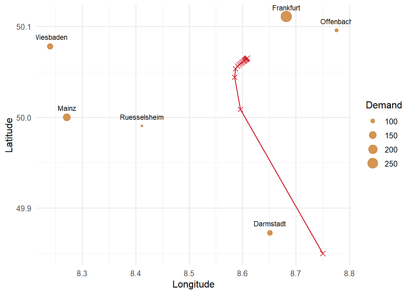
The lecture shows how the algorithm approaches the optimum using a deliberately distant starting point $(x_0, y_0) = (8.75;\ 49.85)$ south-east of Darmstadt. To trace the path, this time we log every iteration:
```{r}
#| label: ch4-weiszfeld-verlauf
#| fig-cap: "Iteration path of the Weiszfeld algorithm from a distant starting point"
daten_w <- data.frame(u = filialen$lon, v = filialen$lat, a = filialen$mu)
x <- 8.75; y <- 49.85                      # distant starting point as in the lecture
verlauf <- tibble(t = 0, x = x, y = y)

for (t in 1:15) {
  d <- sqrt((x - daten_w$u)^2 + (y - daten_w$v)^2)
  g <- daten_w$a / d                        # iteration weights
  x <- sum(daten_w$u * g) / sum(g)
  y <- sum(daten_w$v * g) / sum(g)
  verlauf <- add_row(verlauf, t = t, x = x, y = y)
}

verlauf |>
  mutate(`Step size` = sqrt((x - lag(x))^2 + (y - lag(y))^2)) |>
  head(6) |>
  kable(digits = 4)
ggplot(filialen, aes(lon, lat)) +
  geom_point(aes(size = mu), colour = "#c97a2b", alpha = 0.8) +
  geom_text(aes(label = Filiale), vjust = -1.2, size = 3) +
  geom_path(data = verlauf, aes(x, y), colour = "#d11f2f") +
  geom_point(data = verlauf, aes(x, y), colour = "#d11f2f", shape = 4, size = 2.5) +
  labs(x = "Longitude", y = "Latitude", size = "Demand") +
  theme_minimal(base_size = 12)
```
The very first step already bridges most of the distance; after that, the steps quickly become smaller. The last decimal places, however, stabilise only slowly: before the tolerance of $10^{-6}$ is reached, the algorithm needs several dozen iterations (see above). This is typical of the Weiszfeld algorithm when the optimum lies close to a high-demand customer – here Frankfurt – because its iteration weight $g_i = a_i/d_i$ grows strongly as the distance decreases and the steps become ever shorter.
::: {.vertiefung}
**In depth (theory): Why does the Weiszfeld algorithm converge?**
As a sum of weighted Euclidean norms, the objective function $Z(x,y) = \sum_i a_i\, d_i(x,y)$ is **convex**: each individual distance function $d_i$ is a “cone” with its apex at the customer location, and a non-negatively weighted sum of convex functions is again convex. It follows that every local minimum is also a global minimum — there are no “traps” in which a method could get stuck. If the customer locations do not all lie on a straight line, $Z$ is even strictly convex and the optimum is unique.
The algorithm goes back to @weiszfeld1937point. It can be shown that each iteration step **does not increase** the objective function value: in each step, the update rule minimises a quadratic auxiliary function that touches $Z$ at the current point and lies above $Z$ everywhere (*majorisation principle*). The minimum of the auxiliary function is precisely the weighted mean with the weights $g_i = a_i/d_i$ — i.e. the update rule. Since the objective function value decreases monotonically and is bounded below, the method converges. Special treatment is only necessary if an iteration falls exactly on a customer location ($d_i = 0$, division by zero); in practice, this case is caught, as in `weiszfeld_manual()`, by a small lower bound for $d_i$.
The economic interpretation of the optimality condition $\sum_i a_i (x-u_i)/d_i = 0$ (and analogously for $y$) is also interesting: each customer “pulls” the site in their direction with a force of strength $a_i$, **regardless of their distance**. At the optimum, all pulling forces cancel each other out. This explains the difference from the centre of gravity: there, a customer's pulling force grows with their distance (the derivative of $d_i^2$ is $2 d_i$), so that distant customers influence the result disproportionately.
:::
### Manhattan distances: the weighted median
If the Manhattan distance is used instead of the Euclidean distance, the structure of the problem changes fundamentally – to its advantage. The objective function
$$
Z(x,y) = \sum_{i=1}^n a_i \left(|x-u_i| + |y-v_i|\right)
= \underbrace{\sum_{i=1}^n a_i |x-u_i|}_{\text{depends only on } x} \; + \; \underbrace{\sum_{i=1}^n a_i |y-v_i|}_{\text{depends only on } y}
$$
is additively **separable** in $x$ and $y$: the optimal $x$ coordinate can be determined independently of the optimal $y$ coordinate and vice versa. For each of the two partial sums, a classic result of optimisation applies: the sum of weighted absolute deviations $\sum_i a_i |x - u_i|$ is minimised by the **weighted median** of the $u_i$ – i.e. by the value at which at least half of the (cumulative, sorted by $u_i$) demand is reached.
::: {.definition}
**Definition: Weighted median as the Steiner–Weber solution under Manhattan distance**
Sort the customers in ascending order of their $u_i$ coordinate and determine the cumulative demand $A_j = \sum_{i=1}^{j} a_i$. The optimal $x$ coordinate is the $u_i$ coordinate of the first customer for whom $A_j \geq \tfrac{1}{2}\sum_{i=1}^n a_i$ holds. For $y$, proceed analogously with the $v_i$ coordinates.
:::
Why the weighted median in particular? Consider what happens if the site is shifted a small distance $\Delta$ to the right on the $x$ axis. All customers to the left of the site move $\Delta$ further away, all customers to the right of it move $\Delta$ closer. The objective function thus changes by $\Delta \cdot (A_{\text{left}} - A_{\text{right}})$, where $A_{\text{left}}$ and $A_{\text{right}}$ are the demand totals to the left and right of the site. A shift to the right pays off as long as there is more demand on the right than on the left. As soon as at least half of the total demand lies on the left, a further shift brings no further advantage — that is exactly the weighted median. It is remarkable that only the **order** of the customers on the axis and their demand quantities matter, not the exact distances: a customer who is very far away does not shift the median more strongly than a nearby customer with the same demand.
```{r}
#| label: ch4-manhattan-median
#| echo: true
# Weighted median: smallest value at which the cumulative demand
# reaches at least half of the total demand
gewichteter_median <- function(werte, gewichte) {
  reihenfolge <- order(werte)          # determine sort index (ascending)
  werte <- werte[reihenfolge]          # sort values in this order
  gewichte <- gewichte[reihenfolge]    # sort weights in the same pattern

  kumuliert <- cumsum(gewichte)        # running (cumulative) sum of weights
  schwelle <- sum(gewichte) / 2        # half of total demand

  werte[which(kumuliert >= schwelle)[1]]  # first value that reaches the threshold
}

manhattan_lon <- gewichteter_median(filialen$lon, filialen$mu)
manhattan_lat <- gewichteter_median(filialen$lat, filialen$mu)
c(lon = manhattan_lon, lat = manhattan_lat)
```
The Manhattan solution $(x,y) \approx (`r sprintf("%.4f", manhattan_lon)`; `r sprintf("%.4f", manhattan_lat)`)$ takes the longitude of Darmstadt on the $x$ axis and the latitude of Wiesbaden on the $y$ axis – a typical feature of the weighted median: on **each coordinate axis individually**, it always yields the value of an existing customer location, but because the $x$ and $y$ coordinates are determined independently of each other, it need not coincide overall with a single real store. The centre of gravity and the Weiszfeld optimum, by contrast, practically never coincide exactly with a customer location, since in their case both coordinates are averaged jointly from all stores. Which distance measure is appropriate is ultimately decided by the real transport structure in the sales area – not by the computational effort of the respective method.
## Geographic distances: reality check with the haversine formula
The centre of gravity, the Weiszfeld algorithm and the weighted median implicitly assume that the coordinates $(u_i, v_i)$ are **Cartesian** coordinates in a plane on which Euclidean or Manhattan distances can be meaningfully interpreted. As announced above, we deliberately made this simplifying assumption throughout the section, even though latitude and longitude (WGS84) are actually coordinates on a **curved** surface of the earth, on which one degree of longitude corresponds to a different number of kilometres depending on the latitude. A naive Euclidean distance calculation based on degree coordinates would therefore be misleading at the latest for supra-regional distances – in the Rhine-Main area with its short distances, the error is small, but it should not go unquestioned.
For an exact comparison, the **haversine formula** is used, which calculates the great-circle distance – the shortest connection between two points on the surface of a sphere – from geographic coordinates:
::: {.definition}
**Definition: Haversine distance**
For two points with geographic latitude/longitude $(\varphi_1,\lambda_1)$ and $(\varphi_2,\lambda_2)$ (in radians), the great-circle distance is calculated as
$$
d^{\text{hav}} = 2R \cdot \arctan2\!\left(\sqrt{a},\, \sqrt{1-a}\right),
\qquad
a = \sin^2\!\left(\frac{\Delta\varphi}{2}\right) + \cos(\varphi_1)\cos(\varphi_2)\sin^2\!\left(\frac{\Delta\lambda}{2}\right),
$$
with $R \approx 6{,}371\,\text{km}$ as the mean radius of the earth, $\Delta\varphi = \varphi_2-\varphi_1$ and $\Delta\lambda = \lambda_2-\lambda_1$.
:::
The function `haversine(lat1, lon1, lat2, lon2)` from `R/scm_functions.R` implements exactly this formula and returns the distance in kilometres. As a first application, we calculate the distance between the candidate site Wiesbaden-Erbenheim and the Frankfurt store:
```{r}
#| label: ch4-haversine-beispiel
#| echo: true
haversine(50.0632, 8.2999, 50.1109, 8.6821)
```
### Distance matrix between the candidate sites and the stores
The same function can be used to calculate the complete distance matrix between all three candidate sites and all six stores. Since `haversine()` is vectorised (it accepts vectors of equal length for `lat1`/`lon1`), we can apply it with `sapply()` once per store to the complete vector of the three site coordinates and directly obtain a matrix with one row per site and one column per store:
```{r}
#| label: ch4-distanzmatrix
#| echo: true
# sapply() over the six stores: for each store, haversine() is applied vectorised
# to all three sites at once -> 3x6 distance matrix
distanzmatrix <- sapply(seq_len(nrow(filialen)), function(j) {
  haversine(standorte$lat, standorte$lon, filialen$lat[j], filialen$lon[j])
})
rownames(distanzmatrix) <- standorte$Standort
colnames(distanzmatrix) <- filialen$Filiale
round(distanzmatrix, 1)
```
This distance matrix makes it possible to back up quantitatively the transport proximity that was only assessed qualitatively in the AHP. Multiplying the distance matrix by the demand vector of the stores – again via the matrix product `%*%` – yields, for each site, the demand-weighted total distance to all six stores:
```{r}
#| label: ch4-distanzmatrix-gewichtet
#| echo: true
gewichtete_gesamtdistanz <- distanzmatrix %*% filialen$mu
gewichtete_gesamtdistanz
```
With around `r sprintf("%.0f", gewichtete_gesamtdistanz["Raunheim", 1])` box-kilometres, Raunheim has the **lowest** weighted total distance to the six stores, well ahead of Wiesbaden-Erbenheim (`r sprintf("%.0f", gewichtete_gesamtdistanz["Wiesbaden-Erbenheim", 1])`) and Mainz-Hechtsheim (`r sprintf("%.0f", gewichtete_gesamtdistanz["Mainz-Hechtsheim", 1])`). This purely quantitative indicator thus confirms the ranking that the AHP had derived for the criterion transport proximity (step 2) solely from qualitative pairwise comparisons – a nice example of how qualitative expert assessments and quantitative recalculation can mutually validate each other.
### Reality check for the centre of gravity and the Weiszfeld optimum
Finally, we examine how **realistic** the two continuous optima from the previous section actually are when we drop the planar simplification made at the outset and calculate the true, spherical haversine distance to each store:
```{r}
#| label: ch4-realitaetscheck
#| echo: true
cog_dist <- sapply(seq_len(nrow(filialen)), function(j) {
  haversine(cog_lat, cog_lon, filialen$lat[j], filialen$lon[j])
})
weiszfeld_dist <- sapply(seq_len(nrow(filialen)), function(j) {
  haversine(ergebnis$y, ergebnis$x, filialen$lat[j], filialen$lon[j])
})

realitaetscheck <- tibble(
  Store = filialen$Filiale,
  Demand = filialen$mu,
  `CoG (km)` = round(cog_dist, 1),
  `Weiszfeld (km)` = round(weiszfeld_dist, 1)
)
realitaetscheck |>
  kable(align = "lccc") |>
  kable_styling(full_width = FALSE)
```
The picture is revealing: at around `r sprintf("%.1f", weiszfeld_dist[filialen$Filiale == "Frankfurt"])` km, the Weiszfeld optimum lies considerably closer to the highest-demand store, Frankfurt (280 boxes/day), than the centre of gravity at around `r sprintf("%.1f", cog_dist[filialen$Filiale == "Frankfurt"])` km – conversely, the Weiszfeld optimum moves noticeably further away than the CoG from the smaller stores further west, Wiesbaden and Mainz. The Weiszfeld algorithm thus deliberately “pulls” the site towards the large individual store in Frankfurt, whereas the centre of gravity, as a pure arithmetic mean, reacts less sensitively to individual large demand concentrations but, in return, also lies less close to them. This is not a general superiority of one method or the other, but a good starting point for discussion: how strongly a location method *should* react to individual large customers is ultimately a question of robustness against demand fluctuations and outliers – not solely a question of optimality within the model.
This brings us full circle to the three discrete candidate sites: neither the centre of gravity nor the Weiszfeld optimum lies on one of the three plots actually available – they merely show in which direction of the sales area a production facility would “ideally” shift. The actual location decision at SushiFresh therefore remains a **discrete** choice between the three candidates, for which the AHP in this chapter – narrowly – recommended Mainz-Hechtsheim, while Raunheim is clearly ahead on transport proximity. Whether this qualitative assessment is also confirmed by a pure cost analysis is examined in Chapter [-@sec-standort-2]: there, with the warehouse location problem, we formulate a quantitative optimisation model that explicitly takes into account not only transport costs but also the fixed costs of the plots, and extends the set of candidates by two further sites – and which, as will become apparent, need not necessarily arrive at the same result as the qualitative evaluation carried out here.
## Summary
This chapter has contrasted two fundamentally different approaches to facility location planning, consistently using the example of SushiFresh GmbH and its search for a production site in the Rhine-Main area. **Qualitative methods** – the scoring model and the Analytic Hierarchy Process – evaluate a limited set of discrete alternatives (at SushiFresh: three candidate plots) on the basis of several criteria, including soft ones. The scoring model is simple to apply but suffers from the compensability of its additive structure, which in extreme cases can lead to alternatives with completely different profiles receiving the same overall utility value – as in the case example, in which all three sites achieved exactly the utility value 5.0. The AHP counters this weakness by deriving criteria and alternative weights from pairwise comparisons and by enabling explicit quality control of the expert assessments via the consistency index; in the case example – with a criteria matrix that was, however, not entirely consistent – it narrowly recommended the Mainz-Hechtsheim site.
**Continuous methods** go one step further and search for the optimal site not among given alternatives but as an arbitrary point in a plane. The centre of gravity provides a fast, closed-form approximate solution for this, which, however, only exactly minimises the squared objective function. The Weiszfeld algorithm iteratively solves the actual problem based on linear Euclidean distances and noticeably pulled the SushiFresh site towards the high-demand Frankfurt store. With Manhattan distances, the problem even simplifies to calculating a weighted median per coordinate. Finally, for large-scale geographic applications, the haversine formula provides a more realistic distance measure than the naive Euclidean distance on degree coordinates – and in the case example confirmed both the AHP ranking on transport proximity and the differences in robustness between the centre of gravity and the Weiszfeld optimum.
Both families of methods have in common that they either select the site from a *given* list of alternatives or determine it as an *arbitrary* point in space. In practice, however, the set of realistic sites is often neither completely freely selectable nor limited to a few alternatives preselected by hand, but consists of a larger but finite set of eligible plots or buildings. For this case – **discrete facility location planning** with warehouse location models and network planning heuristics – Chapter [-@sec-standort-2] extends the methodological toolkit with exact and heuristic optimisation methods. There, we return to the SushiFresh case study and examine whether the narrow AHP recommendation in favour of Mainz-Hechtsheim is also confirmed by an explicit cost calculation.
::: {.kontrollfragen}
**Review questions**
1. Explain the five-step procedure of the scoring model and name two of its methodological weaknesses.
2. Why can alternatives with completely different strength–weakness profiles achieve the same overall utility value in the scoring model?
3. Describe the five steps of the AHP. What role does the pairwise comparison matrix play?
4. How is the consistency index (CI) of a pairwise comparison matrix calculated, and below which threshold of the consistency ratio (CR) is a matrix usually considered sufficiently consistent?
5. Derive the formula for the centre of gravity from the minimisation of the weighted squared Euclidean distances.
6. Why does the Weiszfeld algorithm generally provide a better (lower-cost) solution than the centre of gravity, even though both are based on Euclidean distances? What does this mean specifically for the Frankfurt store in the SushiFresh example?
7. How does determining the optimal site under Manhattan distances differ from determining it under Euclidean distances?
8. Why is the direct application of Euclidean distances to geographic coordinates (latitude/longitude) problematic, and what alternative does the haversine formula offer?
9. In the case example, the AHP narrowly recommends the Mainz-Hechtsheim site. Give two reasons why a purely cost-based analysis (as in Chapter [-@sec-standort-2]) could arrive at a different result.
10. In the R code, change the comparison “transport proximity versus skilled labour” from 2 to 1/2. How do the consistency ratio and the ranking of the sites change? Interpret the result.
:::