# Objectives, Trade-offs and Logistics Costs {#sec-logistikkosten}
```{r}
#| label: ch3-setup
#| message: false
#| warning: false
# Tidyverse: dplyr (data manipulation), ggplot2 (graphics), etc.
library(tidyverse)
# kableExtra: formatted HTML/PDF tables (kbl(), kable_styling())
library(kableExtra)

# Load the course colour palette and helper functions (object `cols`)
source("../R/scm_functions.R")
```
::: {.lernziele}
**Learning objectives**
- You can name the system of objectives of logistics and supply chain management and distinguish the key target variables (cost, time, reliability, flexibility/resilience, quality, information).
- You can explain why these objectives are in tension with one another, and interpret the "tetrahedron of trade-offs" as well as objective profiles.
- You can distinguish the most important types of logistics costs (transport, warehousing, inventory holding, handling and shortage costs, among others) and quantify them using examples.
- You can analyse typical logistics trade-off decisions (mode of transport, number of warehouses, safety stock, lot size) by means of opposing cost curves.
- You can use the R pipe operator `|>`, `dplyr::group_by()`/`summarise()` for aggregation and formatted tables with `kableExtra` to evaluate and present cost data.
:::
## From strategy to operational control
The previous chapter focused on the strategic level: which value-creation stages does a company perform itself, which are outsourced, and how must the supply chain be designed so that it matches the competitive strategy (*strategic fit*)? These strategic choices set the framework within which logistics and supply chain management act operationally. This raises the follow-up question: by what exactly is the success of this operational action measured? Which target variables does SCM work with, and what does it cost to achieve these objectives?
This chapter introduces the **system of objectives** of logistics and supply chain management, uses an illustrative "tetrahedron" to show the unavoidable **trade-offs** between cost, speed, quality, flexibility and sustainability, and identifies the most important **types of logistics costs**. Finally, several numerical examples — from the banana value chain to the Apple iPod — show how logistics costs are made up in practice and how they can be analysed systematically with R.
## Objectives of supply chain management
Supply chain management designs material, information and financial flows across company boundaries. Every design decision — for example on locations, inventories, modes of transport, capacities or suppliers — affects several target variables at once. A low-cost network may lead to long delivery routes. High delivery readiness may increase safety stocks. Strong centralisation may reduce inventories and depreciation, but at the same time increase distances to customers.
A well-founded decision therefore requires more than asking which alternative causes the lowest immediate costs. It demands a transparent assessment of economic, performance-related, risk-related and environmental effects. This chapter develops the concepts and modelling logic on which the following chapters on facility location planning, uncertainty and inventory control build.
## Systems of objectives in companies: a positioning
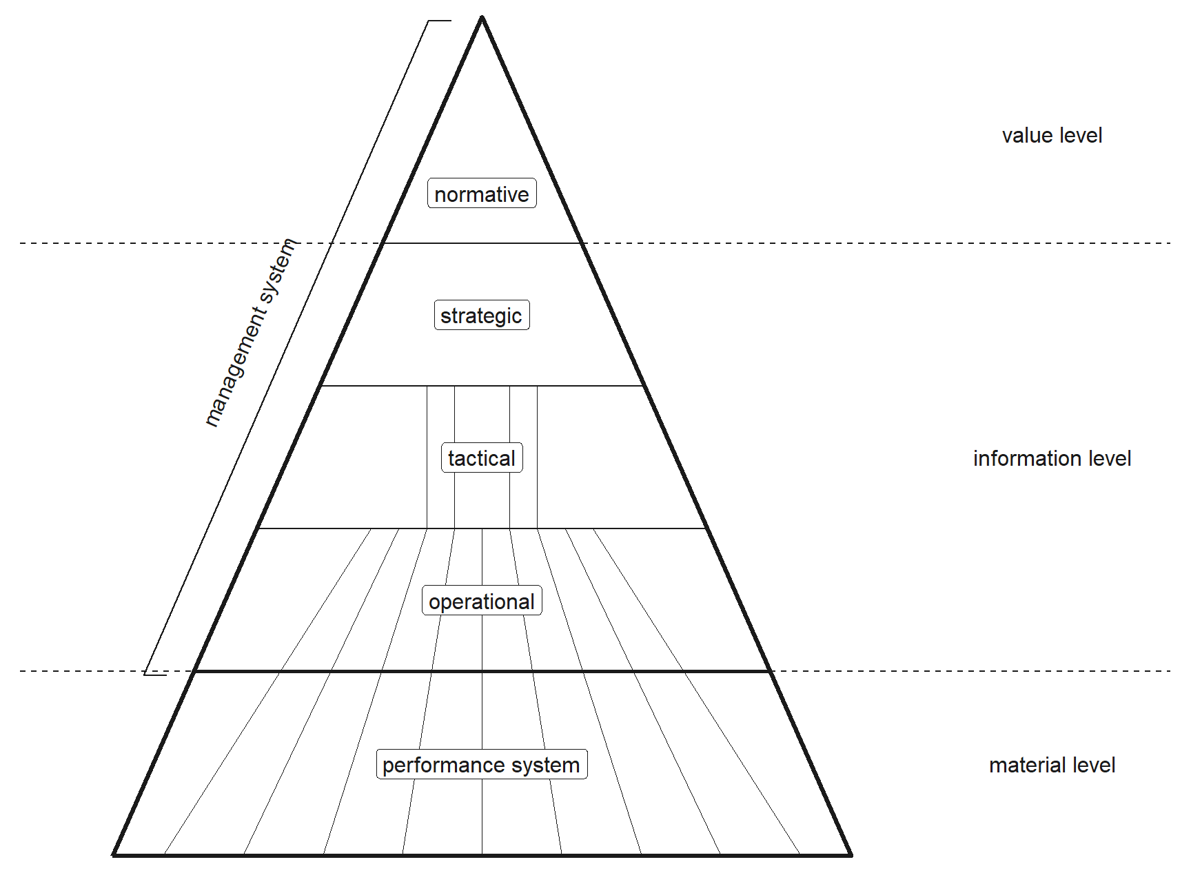
Before we turn to logistics-specific objectives, it is worth taking a brief look at the structure of corporate systems of objectives as a whole. Every company has a hierarchically structured management system: at the **normative level**, fundamental values, the corporate constitution and the corporate culture are defined; at the **strategic level**, long-term success potentials are built up (this was the subject of Chapter [-@sec-strategic-fit]); finally, at the **operational level**, day-to-day business is controlled in such a way that the strategic targets are met [@dyckhoff1998grundzuege].
```{r}
#| label: fig-management-levels
#| echo: false
#| fig-cap: "Levels of the management system above the performance system (after @dyckhoff1998grundzuege)"
#| fig-width: 9
#| fig-height: 6.6
#| out-width: "75%"
#| fig-align: center
plot_management_pyramid()
```
@fig-management-levels also shows how the levels relate to each other: the normative level belongs to the *value level*, the strategic, tactical and operational levels to the *information level*, and all of them steer the *performance system* at the *material level*, where goods are actually procured, produced and distributed.
Each of these levels has its own objectives — from very general, long-term mission statements to very concrete, short-term measurable key figures. Logistics and SCM objectives are typically located at the strategic to operational level: they are derived from higher-level corporate objectives (e.g. profitability, growth, customer satisfaction), but are concrete enough to serve as decision criteria in day-to-day business.
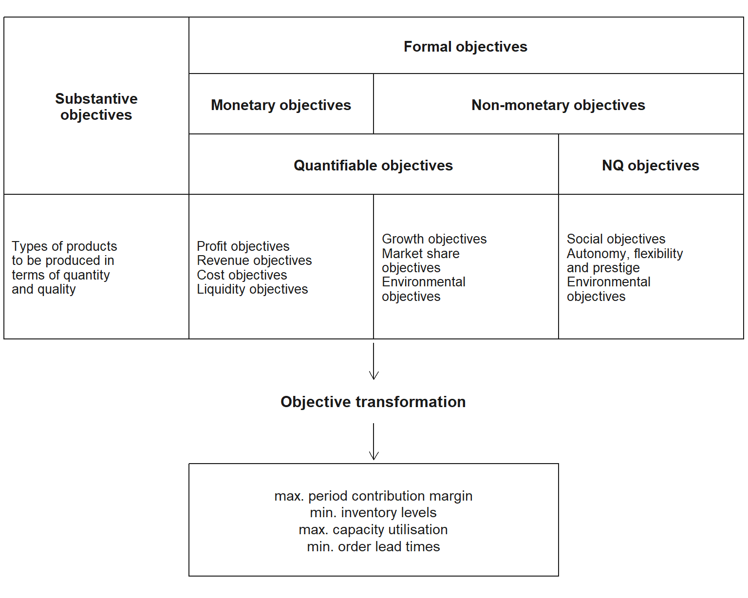
A common classification distinguishes **substantive objectives** (what is to be produced, in which quantities and qualities) from **formal objectives**, which measure the success of this activity. Formal objectives are either monetary (profit, revenue, costs, liquidity) or non-monetary; the latter can be quantifiable (growth, market share, environmental objectives) or non-quantifiable (social objectives, autonomy, flexibility, prestige). For decision-making, these objectives must be transformed into operational target metrics such as a maximum period contribution margin or minimum inventory levels (@fig-objective-types).
```{r}
#| label: fig-objective-types
#| echo: false
#| fig-cap: "Substantive and formal objectives and their transformation into operational target metrics [after @buscher2013produktion, p. 12]"
#| fig-width: 8
#| fig-height: 6.4
#| out-width: "75%"
#| fig-align: center
plot_objective_types()
```
This classification is more than an academic exercise: it explains why logistics decisions are almost never made "in a vacuum". A decision on the number of distribution warehouses, for example, is an operational to strategic decision, but it only makes sense if it fits the company's overarching service strategy. A company that has opted for cost leadership at the strategic level (cf. Chapter [-@sec-strategic-fit]) will tend to set different target aspiration levels at the operational level than a company that relies on differentiation through speed. The system of objectives of logistics is therefore not an end in itself, but the operational "translation" of the competitive strategy into measurable variables.
::: {.definition}
**Definition: Objective**
An **objective** describes a desired future state that is characterised by a **target variable** (the *what*, e.g. "delivery time"), an **aspiration level** (the *how much*, e.g. "a maximum of 24 hours") and a **time reference** (the *by when*). Objectives serve as a yardstick against which decision alternatives are evaluated and degrees of goal achievement are measured.
:::
### Economic efficiency
Economic efficiency means using the resources employed to provide a service efficiently. In supply chains, this includes in particular procurement, production, warehousing, transport, transhipment, information and coordination costs. What matters is not isolated individual costs, but the costs of the entire system. A measure that lowers local transport costs may, for example, cause higher inventories, longer lead times or poorer service levels elsewhere.
The total-cost perspective is often referred to as *total cost of ownership* or *total logistics cost* thinking. It requires decisions to be evaluated along the entire chain and not only from the perspective of a single function or a single company.
### Service and time
For customers, logistics performance is reflected above all in availability, delivery time, delivery reliability, flexibility and information quality. Typical key figures are the degree of delivery readiness, complete and on-time delivery, and mean lead time.
A high service level can rarely be achieved free of charge. Shorter delivery times often require more warehouse locations, additional capacity, higher safety stocks or faster transport modes. The central managerial task is to determine the desired performance level explicitly and to make the resources required for it visible.
### Resilience and risk
Supply chains are exposed to disruptions, for example from demand fluctuations, supplier failures, capacity bottlenecks, natural events or infrastructure interruptions. Resilience describes the ability of a network to absorb such disruptions, adapt and restore its performance.
Resilience can be improved through redundancy, alternative sources of supply, flexible capacity, regional diversification, transparency and appropriate safety stocks. Such measures often increase immediate costs. However, they can make economic sense if they reduce expected disruption costs, lost revenue or reputational damage.
### Sustainability
Sustainability extends the system of objectives to include environmental and social effects. This chapter initially focuses on the environmental effects of logistics decisions: greenhouse gas emissions, energy and resource consumption, land use, air pollutants, waste and spoilage. Social aspects — such as working conditions, safety and regional value creation — are also relevant, but are not converted into a single quantitative measure here.
Sustainability is not an isolated additional criterion. It changes how locations, transport routes, inventories, packaging, production quantities and procurement structures are evaluated. In many supply chains, significant environmental impacts arise not in the company's own operations, but at upstream suppliers, transport service providers or in the use and take-back phase of products.
## Target metrics in logistics and supply chain management
Traditionally, the performance of logistics and supply chain management is assessed using a manageable set of **target metrics**. Six variables appear in almost every logistics textbook and together form a wheel whose spokes influence one another:
- **Delivery time**: the time span between the customer placing the order and the actual fulfilment of the order (receipt of goods by the customer). Short delivery times increase customer satisfaction, but often require higher inventories or more expensive modes of transport.
- **Delivery reliability**: the relationship between the promised and the actually achieved delivery date. High delivery reliability means that commitments are reliably kept — regardless of how long the promised period is.
- **Delivery quality**: the share of orders that were executed correctly in terms of both quantity and quality (no wrong or missing deliveries, no transport damage).
- **Flexibility/resilience**: the ability to implement short-term changes in quantities, dates or product specifications, or to recover quickly from disruptions (supply shortages, demand shocks).
- **Information**: the quality and transparency of the information available throughout order processing — for example shipment tracking or reliable inventory data.
- **Cost**: the efficiency with which all these services are provided, measured by the total costs of the logistics activities.
These six target variables are not independent of one another. On the contrary: their interplay — more precisely, their *contradiction* — is the actual core of logistics management, as the following section shows.
In addition to these "classical" economic target variables, **environmental and social objectives** have increasingly come to the fore in recent years: the reduction of greenhouse gas emissions along the chain, the careful use of resources or compliance with minimum social standards at suppliers. These objectives are not simply added alongside the existing system of objectives, but further intensify the existing trade-offs — a lower-emission rail connection is often slower than road haulage, and a regional rather than global supplier may be more expensive but environmentally more advantageous. A complete treatment of this third and fourth dimension of objectives would go beyond the scope of this chapter; it is, however, noted here as an outlook and is covered in depth by @dyckhoff2008nachhaltige.
## The tension between logistics objectives: dimensions of objectives and the tetrahedron
If one tried to maximise or minimise each of the six target variables independently, the result would be a logistics system with perfect delivery time, perfect delivery reliability, perfect quality, maximum flexibility and full transparency — at minimum cost. Such a system does not exist. As a rule, any improvement in one target variable comes at the expense of at least one other. This is referred to as a **trade-off (goal conflict)**.
::: {.definition}
**Definition: Trade-off (goal conflict)**
A **goal conflict** exists when the improvement of one target variable (e.g. shorter delivery time) necessarily entails the deterioration of at least one other target variable (e.g. higher costs). Goal conflicts cannot be "resolved", but can only be handled through a deliberate weighing-up — a **trade-off**.
:::
::: {.vertiefung}
**In depth (theory): Relationships between objectives and Pareto efficiency**
Managerial decision theory distinguishes three types of relationship between two objectives [@dyckhoff1998grundzuege]: **complementary** objectives support each other (better delivery quality, for example, reduces complaint costs and thus logistics costs), **indifferent** objectives do not influence each other, and **competing** objectives are in conflict. It is important to note that the type of relationship is not "given by nature", but depends on the range of alternatives under consideration: as long as a logistics system contains waste (such as empty runs or duplicated inventories), cost and delivery time can often be improved **simultaneously** — in this range the objectives behave in a complementary way. Only when all such improvements have been exhausted does the relationship become competitive.
Formally, an alternative is called **Pareto-efficient** (or non-dominated) if there is no other feasible alternative that is better in at least one objective and worse in none. The set of all Pareto-efficient alternatives forms the **efficient frontier** — the same concept that was introduced in Chapter [-@sec-strategic-fit] as the cost–responsiveness frontier. Genuine trade-offs exist only *on* this frontier. This gives rise to two management tasks that should be clearly separated: first, bringing an inefficient system up to the frontier (here there is no trade-off, only potential for improvement), and second, choosing a position on the frontier that matches the competitive strategy (here a trade-off is unavoidable). The objective profiles below are essentially nothing other than different positions on such a multidimensional efficient frontier.
:::
For illustration, the system of objectives is often reduced to four central, highly condensed dimensions: **quality**, **speed**, **cost** and **flexibility/resilience**. If these four dimensions are represented as the four vertices of a tetrahedron (a triangular pyramid), the tension becomes immediately visible: each edge of the tetrahedron connects two target variables between which a trade-off must be made, and no real logistics system can be positioned "perfectly" in all four corners at the same time.
```{r}
#| label: ch3-tetraeder
#| fig-cap: "The tetrahedron of trade-offs: quality, speed, cost and flexibility/resilience are in mutual tension."
#| fig-alt: "Three-dimensional pyramid (tetrahedron) with the four vertices quality, speed, cost and flexibility/resilience."
library(plotly)

# Four vertices of the tetrahedron: 1-3 form the base, 4 the apex
eckpunkte <- data.frame(
  ziel = c("Quality", "Speed", "Cost", "Flexibility / resilience"),
  x = c(-3.8, 0.0, 3.8, 0.0),
  y = c(-2.2, 3.2, -2.2, 0.0),
  z = c(0.0, 0.0, 0.0, 4.2)
)

# Four triangular faces: base (0,1,2) and three side faces to the apex (3)
flaechen_i <- c(0, 0, 0, 1)
flaechen_j <- c(1, 2, 3, 2)
flaechen_k <- c(2, 3, 1, 3)

# Build the 3D graphic with plotly: faces (mesh3d), edges (lines), labels
fig_tetraeder <- plot_ly() |>
  add_trace(
    type = "mesh3d",
    x = eckpunkte$x, y = eckpunkte$y, z = eckpunkte$z,
    i = flaechen_i, j = flaechen_j, k = flaechen_k,
    intensity = c(0.20, 0.55, 0.85, 1.00),
    colors = c(cols$mid, cols$atp, cols$strat, cols$top),
    opacity = 0.78, flatshading = TRUE, showscale = FALSE,
    hoverinfo = "skip"
  ) |>
  add_trace(
    type = "scatter3d", mode = "markers+text",
    x = eckpunkte$x, y = eckpunkte$y, z = eckpunkte$z,
    text = eckpunkte$ziel,
    textposition = "top center",
    marker = list(size = 6, color = cols$border),
    textfont = list(size = 13, color = cols$text),
    hovertemplate = "%{text}<extra></extra>",
    showlegend = FALSE
  ) |>
  layout(
    scene = list(
      xaxis = list(visible = FALSE), yaxis = list(visible = FALSE),
      zaxis = list(visible = FALSE), bgcolor = "white"
    ),
    paper_bgcolor = "white",
    margin = list(l = 0, r = 0, b = 0, t = 0)
  )

fig_tetraeder
```
Specific logistics systems can then be characterised as **objective profiles** within this area of tension. An express courier service, for example, positions itself close to the "speed" corner — at the expense of cost. A bulk sea-freight service geared towards cost efficiency, by contrast, lies close to the "cost" corner — at the expense of delivery time. A supplier in just-in-sequence production, in turn, has to operate on the edge between flexibility and speed, as it must respond to short-term changes in call-offs *and* still deliver exactly on schedule.
Instead of the four condensed dimensions, the four original variables **delivery time**, **delivery reliability**, **delivery flexibility** and **logistics costs** can also be shown in a so-called **objective profile chart** (also known as a radar or spider chart). Each axis represents a target variable; a specific system is represented by a polygon whose vertices correspond to the values achieved. If several systems (or system alternatives) are compared in this way, differences in strategic positioning become immediately visible — a system with a "pointed", one-sided profile pursues a clear focus strategy, whereas a more balanced profile relies on a compromise between the objectives.
```{r}
#| label: ch3-zielprofile
#| fig-cap: "Objective profiles: four logistics systems with different positioning between short delivery times, high delivery reliability, great delivery flexibility and low logistics costs."
#| fig-alt: "Radar chart with four axes (delivery time, delivery reliability, delivery flexibility, logistics costs) and four plotted objective profiles."
library(plotly)

# Four target variables on a scale from 0 to 10; each profile is a polygon.
# The first axis is repeated at the end so that the polygon closes.
achsen <- c("short delivery time", "high delivery reliability",
            "great delivery flexibility", "low logistics costs")

zielprofile <- tibble::tribble(
  ~profil,    ~lieferzeit, ~zuverlaessigkeit, ~flexibilitaet, ~kosten,
  "Profile 1",         5.8,               8.7,            5.8,     1.8,
  "Profile 2",         7.6,               3.2,            8.6,     3.2,
  "Profile 3",         9.3,               4.9,            1.5,     5.0,
  "Profile 4",         3.6,               1.5,            3.6,     8.2
)

# Radar chart with plotly (scatterpolar): one trace per objective profile
fig_zielprofile <- plot_ly(type = "scatterpolar", fill = "toself")

for (i in seq_len(nrow(zielprofile))) {
  werte <- as.numeric(zielprofile[i, -1])
  fig_zielprofile <- fig_zielprofile |>
    add_trace(
      r = c(werte, werte[1]),               # repeat first axis -> polygon closes
      theta = c(achsen, achsen[1]),
      name = zielprofile$profil[i],
      opacity = 0.35
    )
}

fig_zielprofile <- fig_zielprofile |>
  layout(
    polar = list(radialaxis = list(visible = TRUE, range = c(0, 10))),
    paper_bgcolor = "white"
  )

fig_zielprofile
```
Both representations — tetrahedron and objective profile — convey the same message: logistics and SCM decisions are almost always **trade-off decisions**. The point is not to find "the best" system per se, but to choose the objective profile that best fits the overarching competitive strategy — a direct continuation of the strategic-fit idea discussed in Chapter [-@sec-strategic-fit] [@chopra2025supply].
::: {.r-exkurs}
**R aside: The pipe operator `|>`**
In the previous chapters, you have mostly written individual R commands one after the other on separate lines or nested function calls inside one another. With multi-step data processing — "take the data, filter it, group it, summarise it, sort it" — nesting quickly becomes confusing. The **pipe operator** `|>` (read as "then") solves this problem: it takes the result on its left-hand side and passes it as the *first* argument to the function on its right-hand side.
```{r}
#| label: ch3-pipe-demo
# Without pipe: function calls are nested from the inside out
kosten <- c(120, 340, 95, 410, 180)
round(mean(sort(kosten, decreasing = TRUE)), 1)
# With pipe: the same calculation, but readable in the order
# in which it is thought through ("take kosten, then sort, then...")
kosten |>
  sort(decreasing = TRUE) |>
  mean() |>
  round(1)
```
The pipe operator does *not* change what is calculated — only how easy it is to follow the calculation. From now on we will use it throughout, especially in combination with the `dplyr` functions `filter()`, `mutate()`, `group_by()` and `summarise()`, which you have already met in Chapter [-@sec-strategic-fit] or will meet below. A pipe chain then reads almost like a sentence: *"Take the cost data, group it by cost type, and summarise it into totals."*
:::
## Logistics costs as a basis for decision-making
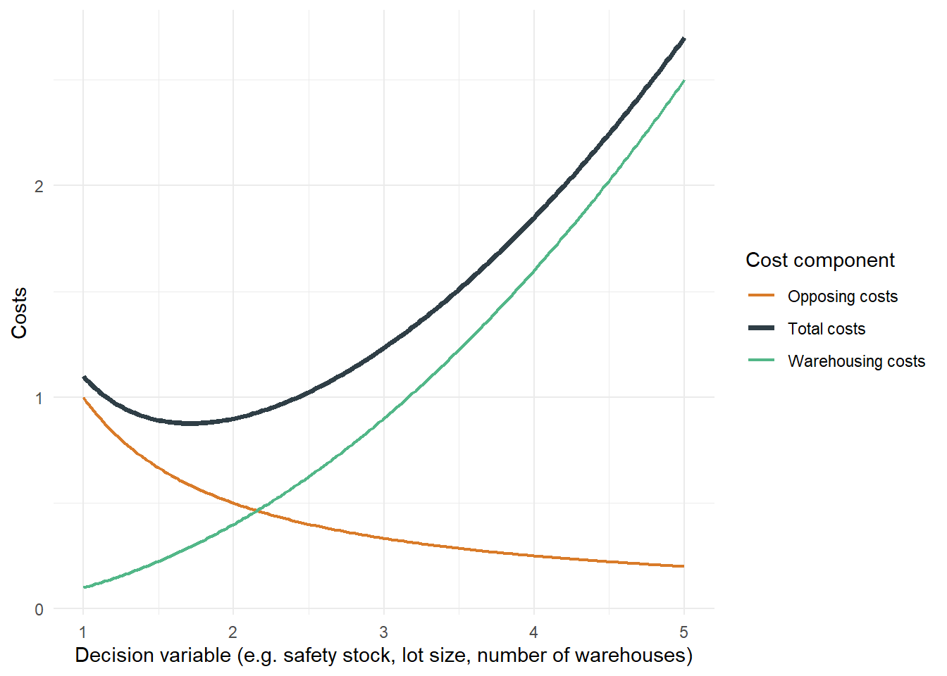
The cost perspective deserves closer attention because it appears as the "opponent" of time, quality and flexibility in practically every trade-off. In many areas of logistics, two (or more) cost components face each other that behave in *opposite* directions with respect to the same decision variable: if one type of cost rises, the other falls — and vice versa. Because both effects act simultaneously, the **total costs** follow a U-shaped curve with a (at least theoretical) cost minimum.
Formally, such a relationship can often be described by a cost function of the form
$$
K(x) = \underbrace{a \cdot x^2}_{\text{increasing cost type}} + \underbrace{\frac{b}{x}}_{\text{decreasing cost type}}, \qquad x > 0
$$
where $x$ is the decision variable (e.g. safety stock, lot size, number of warehouses) and $a, b > 0$ are cost parameters. The minimum of this function is obtained by setting the first derivative to zero:
$$
K'(x) = 2a x - \frac{b}{x^2} \stackrel{!}{=} 0 \quad \Longrightarrow \quad x^* = \left(\frac{b}{2a}\right)^{1/3}
$$
This pattern — one increasing and one decreasing cost component whose sum has a minimum — appears again and again in logistics in similar form. The interpretation of the parameters $a$ and $b$ is important here: they are not arbitrary constants, but represent real cost rates (e.g. interest rate and warehousing cost rate per unit for $a$, set-up or shortage cost rate for $b$) and would have to be estimated from cost accounting in practice. Depending on the decision situation, *which* type of cost rises and which falls also changes — but the basic mathematical pattern remains the same. Four typical examples:
1. **Choice of transport mode**: faster modes of transport (air) cause higher direct transport costs, but reduce the costs of capital tied up in inventory (shorter transit time $\rightarrow$ less inventory in transit). Slower modes of transport (sea, rail) are cheaper per unit, but tie up capital in inventory for longer.
2. **Number of warehouses**: more warehouse locations increase the costs of warehousing and replenishment (more fixed costs, more safety stock), but reduce the transport costs of delivery to customers (shorter "last mile").
3. **Level of safety stock**: a higher safety stock increases warehousing costs (capital tie-up, storage space), but reduces the expected shortage costs (lost revenue, contractual penalties, damage to reputation in the event of delivery failures).
4. **Lot size**: larger order quantities or production lots increase warehousing costs (more average inventory), but reduce set-up or ordering costs (fewer orders/changeovers per period).
```{r}
#| label: ch3-tradeoff-plot
#| fig-cap: "Basic pattern of a logistics trade-off decision: two opposing cost components add up to a U-shaped total cost curve with a cost minimum."
#| fig-alt: "Line chart with three curves: a decreasing one, an increasing one and the U-shaped sum curve with a minimum."
# Decision variable x (e.g. safety stock, lot size, number of warehouses)
x <- seq(1, 5, length.out = 200)

# Two opposing cost components
kosten_a <- 0.1 * x^2   # e.g. warehousing/inventory costs: increase with x
kosten_b <- 1 / x       # e.g. shortage/set-up/transport costs: decrease with x
kosten_gesamt <- kosten_a + kosten_b

tradeoff_df <- tibble(
  x = x, Lagerkosten = kosten_a, Gegenkosten = kosten_b, Gesamtkosten = kosten_gesamt
) |>
  pivot_longer(-x, names_to = "kostenart", values_to = "kosten")

# English legend labels for the (German) internal keys
kosten_labels <- c(
  Lagerkosten = "Warehousing costs", Gegenkosten = "Opposing costs", Gesamtkosten = "Total costs"
)

ggplot(tradeoff_df, aes(x = x, y = kosten, color = kostenart, linewidth = kostenart)) +
  geom_line() +
  scale_color_manual(values = c(
    Lagerkosten = cols$mid, Gegenkosten = cols$atp, Gesamtkosten = cols$border
  ), labels = kosten_labels) +
  scale_linewidth_manual(values = c(Lagerkosten = 0.8, Gegenkosten = 0.8, Gesamtkosten = 1.3),
                         labels = kosten_labels) +
  labs(
    x = "Decision variable (e.g. safety stock, lot size, number of warehouses)",
    y = "Costs", color = "Cost component", linewidth = "Cost component"
  ) +
  theme_minimal()
```
However illustrative this basic pattern is, in practice it often remains only an approximation. The actual **transparency of cost functions** is often severely limited, for several reasons:
- **Data availability**: many cost components (especially shortage costs) are difficult to observe because lost revenue or damage to reputation does not appear directly in the accounts.
- **Intertemporal attributability**: investment decisions (e.g. building a new warehouse) have an effect over several periods; which share of the costs is to be "attributed" to which period is a normative, not a purely technical question.
- **Cost responsibility**: in complex supply chains with several actors, it is often unclear who ultimately bears which costs — the manufacturer, the logistics service provider or the retailer.
- **Stochasticity**: demand, lead-time and disruption risks are subject to randomness; cost functions based on expected values conceal the variability around this expected value.
Despite these limitations, the basic pattern "two opposing cost components, one optimum" is a central thinking tool in logistics management. We will encounter it again in the following chapters in a more concrete, formalised form — for example when determining the optimal order quantity (EOQ model) or when choosing the optimal safety stock under demand uncertainty.
::: {.r-exkurs}
**R aside: Vectorised cost calculations**
R is **vectorised** from the ground up: arithmetic operations automatically apply to every element of a vector, without the need for an explicit loop (`for`). This is particularly practical when total costs are to be made up of several cost components, each of which is available for different periods, locations or products.
```{r}
#| label: ch3-vektor-kosten
# Monthly cost components of a warehouse location (in EUR thousand)
transportkosten <- c(42, 38, 45, 51, 47, 39)
lagerkosten     <- c(18, 19, 17, 20, 21, 18)
fehlmengenkosten <- c(3, 1, 6, 2, 0, 4)

# Total costs per month: element-wise sum of the three vectors --
# R automatically adds element 1 to element 1, element 2 to element 2, etc.
gesamtkosten <- transportkosten + lagerkosten + fehlmengenkosten
gesamtkosten
# Share of shortage costs in total costs per month, in per cent
fehlmengenkosten / gesamtkosten * 100
# Key figures across all six months
c(
  Total = sum(gesamtkosten),
  Mean = mean(gesamtkosten),
  Maximum = max(gesamtkosten)
)
```
Without vectorisation, one would have to write a loop over the six months for each of these calculations. Since R performs vector operations "element-wise", a single expression is sufficient — shorter, more readable and less error-prone.
:::
## Types of logistics costs at a glance
Now that the basic pattern of the trade-off has been clarified, it is worth taking a more systematic look at **logistics costs** themselves.
::: {.definition}
**Definition: Logistics costs**
**Logistics costs** are the valued consumption of goods and services for the purpose of providing logistics services — that is, all activities that make goods available in the right quantity and quality, at the right place and at the right time [@schulte2001material].
:::
In the literature and in practice, a rough classification into five to six main categories has become established, which follows directly from the trade-off decisions discussed in the previous section:
- **Transport costs**: costs for the physical transport of goods between two points of the supply chain — depending on the mode of transport, distance, quantity transported and desired speed. They include both the actual freight costs and costs for transhipment and pre-/on-carriage.
- **Warehousing/handling costs**: costs for warehousing in the narrower sense (rent or imputed depreciation of the storage space, energy, staff for putaway, retrieval and relocation) as well as for order picking and internal transport. As a rule, these costs increase with the number of warehouse locations and with the average inventory held.
- **Inventory holding costs** (also: capital tie-up costs): costs arising from the capital tied up in inventory — imputed interest on the tied-up capital, insurance, depreciation/obsolescence and shrinkage. They are often expressed as a percentage of the average inventory value (typical orders of magnitude: 15–30% p.a.).
- **Shortage costs**: costs incurred when demand cannot be served (on time) — lost contribution margin, contractual penalties, expediting costs for replacement deliveries and long-term damage to reputation, which may be reflected in future lost orders. Shortage costs are particularly difficult to quantify because part of them (loss of image) only becomes apparent with a considerable delay.
- **Set-up/ordering costs**: fixed, quantity-independent costs per order or set-up (staff and administrative effort for order processing or machine changeover in production). They are incurred at the same level regardless of the quantity ordered or produced — one reason why larger, less frequent lots reduce this type of cost per unit.
- **Packaging and information costs**: costs for packaging material (including protection and load securing) and for the IT handling of order processing (order entry, shipment tracking, EDI interfaces to customers and suppliers).
These cost types correspond closely to the four trade-off examples from the last section: the choice of transport mode primarily concerns transport vs. inventory holding costs, the number of warehouses concerns warehousing vs. transport costs, safety stock concerns inventory holding vs. shortage costs, and lot size concerns warehousing vs. set-up costs. A central concern of supply chain costing (cost accounting along the entire chain) is to consider these cost types not in isolation for each company, but **across the chain** — because local cost optimisation at one actor can lead to higher costs elsewhere in the chain [@guenther2012produktion; @thonemann2023operations].
## Example: value creation and logistics costs in the banana chain
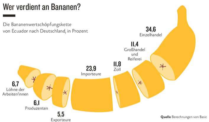
The value chain of bananas from Ecuador to Germany (@fig-bananenkette) shows how strongly logistics and trade margins can shape the final price of a product. Of every euro that consumers pay for a banana in German retail, only around 6.1% remains with the producers and 6.7% as wages for workers on the ground — while importers (23.9%) and retailers (34.6%) capture the largest part of the margin.
{#fig-bananenkette}
This distribution can be reproduced in R and analysed systematically — a good opportunity to introduce two central `dplyr` tools: `group_by()` and `summarise()`.
::: {.r-exkurs}
**R aside: Aggregation with `group_by()` and `summarise()`**
Cost data are often available in a "long" table — one row per individual item — and one wants to **group** them by a characteristic and calculate a key figure (sum, mean, count, …) for each group. This is exactly what `dplyr::group_by()` and `dplyr::summarise()` do in combination:
1. `group_by(spalte)` conceptually divides the data set into subgroups based on the values of `spalte`.
2. `summarise(neue_spalte = funktion(...))` calculates one or more summary key figures for **each group** and returns a new, more compact table — one row per group.
```{r}
#| label: ch3-bananen-gruppieren
# Banana value chain: share of each actor in the final price (in per cent)
bananenkette <- tibble::tribble(
  ~akteur,                    ~kategorie,        ~anteil_prozent,
  "Workers' wages",           "Country of production",       6.7,
  "Producers",                "Country of production",       6.1,
  "Exporters",                "Country of production",       5.5,
  "Importers",                "Trade",                      23.9,
  "Customs",                  "Trade",                      11.8,
  "Wholesale and ripening",   "Trade",                      11.4,
  "Retail",                   "Trade",                      34.6
)

# Pipe + group_by + summarise: "Take the banana chain, group by
# category, and sum the share of the final price per category."
bananenkette |>
  group_by(kategorie) |>
  summarise(
    anteil_gesamt = sum(anteil_prozent),
    anzahl_akteure = n()
  )
```
The result makes the central message of the figure tangible in a single number: only around 18.3% of the final price remains in the country of production (across three actors), while 81.7% goes to trade, customs and distribution in the destination country (across four actors). `group_by()`/`summarise()` works on the same principle for logistics costs: if, for example, one groups by cost type (transport, warehousing, inventory, shortages) instead of by chain category, one obtains an overview of cost types in exactly the same way — an analysis that is carried out routinely in every logistics controlling department.
:::
## Formatted tables: the example of logistics cost shares
Raw tables as in the last R aside are practical for interactive analysis, but are often too plain for presentation in a report or a presentation. The `kableExtra` package makes it possible to format tables professionally with just a few additional commands.
The application example is a comparison of the share of logistics costs (LC) in the selling price for five very different products — from jeans made in Bangladesh to a mobile phone assembled in China and shipped by air freight.
::: {.r-exkurs}
**R aside: Formatted tables with `kableExtra`**
`kableExtra` builds on `knitr::kable()` and adds styling options. The typical workflow is: prepare data with `dplyr` $\rightarrow$ convert into a table with `kbl()` (short for "kable") $\rightarrow$ format with `kable_styling()`.
```{r}
#| label: ch3-kableextra-demo
# Logistics cost shares of selected products (data roughly based on
# practice-oriented calculation examples, rounded)
produktkosten <- tibble::tribble(
  ~produkt,          ~verkaufspreis_eur, ~direkte_lk_eur, ~indirekte_lk_eur,
  "Jeans",                        12.92,            1.89,              3.19,
  "Blouse",                      129.30,            2.77,             16.81,
  "Ford Focus",                12932.03,         1175.00,            106.00,
  "Electric toothbrush",         112.07,            8.19,              7.08,
  "Mobile phone",                120.69,            5.95,              9.03
)

# Calculate total logistics costs and their share of the selling price
produktkosten <- produktkosten |>
  mutate(
    lk_gesamt_eur = direkte_lk_eur + indirekte_lk_eur,
    lk_anteil_prozent = round(lk_gesamt_eur / verkaufspreis_eur * 100, 1)
  )

# Formatted table: kbl() creates the table, kable_styling()
# formats it (e.g. striped rows, compact width)
produktkosten |>
  select(Product = produkt, `Price (€)` = verkaufspreis_eur,
         `Total LC (€)` = lk_gesamt_eur, `LC share (%)` = lk_anteil_prozent) |>
  kbl(digits = 2, caption = "Logistics cost shares of selected products") |>
  kable_styling(bootstrap_options = c("striped", "hover", "condensed"),
                full_width = FALSE)
```
:::
The table shows a remarkable range: while logistics costs for the Ford Focus are relatively low at around 9.9% of the selling price (because the vehicle price itself is very high), they account for almost 40% of the selling price for the comparatively cheap jeans. The reason lies in the **ratio of product value to transport effort**: jeans are transported over long distances by sea freight and are nevertheless a "low-value" product, so that the logistics costs (small in absolute terms) make up a large share of the likewise small selling price. The opposite is true for the car: even though logistics costs are high in absolute terms (global sourcing, several transport stages), the vehicle value is so high that the percentage share remains low. This observation is an important principle for practice: **the significance of logistics costs depends crucially on the value-to-weight or value-to-volume ratio of a product** — a relationship that also influences the location decisions in the next chapter.
## Supply chain costing: the example of the Apple iPod
A particularly illustrative case example of **supply chain costing** — that is, the analysis of the distribution of costs and value added along an entire, globally distributed chain — is provided by Apple's video iPod (30 GB), as reconstructed in the study by Dedrick, Kraemer and Linden [@dedrick2012usitc].
The value chain comprises four process stages: **procurement**, **production**, **distribution** and **sales**. Components such as the hard disk and display come from Japan, memory chips from Korea, the processor and flash memory from the USA, and other parts (including the battery) from other countries. Final assembly takes place in China, while distribution and retail run via the USA before the product reaches US end customers.
The cost structure can be summarised as follows: the purchased components add up to 97 + 3 + 16 + 24 = 140 US dollars. Assembly in China costs an additional 4 US dollars, and distribution and retail in the USA account for around 75 US dollars. Together this gives 140 + 4 + 75 = 219 US dollars, which the study reports as "manufacturing costs" from Apple's perspective — the term is thus used broadly here and covers the entire chain up to the shelf. With a selling price of 299 US dollars, Apple is left with a contribution margin of 80 US dollars in absolute terms, or around 26% of the selling price in relative terms.
```{r}
#| label: ch3-ipod-kostenrechnung
# Cost items of the Apple video iPod (30 GB), in US dollars
ipod_kosten <- c(
  Komponenten_Japan  = 97,
  Komponenten_Korea  =  3,
  Komponenten_USA    = 16,
  Komponenten_Sonstige = 24,
  Montage_China      =  4,
  Distribution_Handel = 75
)

# Vectorised summation: total manufacturing costs
herstellungskosten <- sum(ipod_kosten)
herstellungskosten
verkaufspreis <- 299
deckungsbeitrag_abs <- verkaufspreis - herstellungskosten
deckungsbeitrag_rel <- deckungsbeitrag_abs / verkaufspreis * 100

# Overview of key figures
tibble::tibble(
  Manufacturing_costs = herstellungskosten,
  Selling_price = verkaufspreis,
  Contribution_margin_absolute = deckungsbeitrag_abs,
  Contribution_margin_relative_percent = round(deckungsbeitrag_rel, 1)
) |>
  kbl(digits = 1, caption = "Cost accounting for the Apple video iPod (30 GB)") |>
  kable_styling(bootstrap_options = c("striped", "condensed"), full_width = FALSE)
```
What is remarkable about this example is that the distribution and retail costs (75 US dollars) are almost as high as *all* component costs combined (140 US dollars), and final assembly in China accounts for only a minimal share at 4 US dollars. This pattern is typical of global electronics supply chains: most of the value added — and a considerable part of the costs — arises not in manufacturing itself, but in procurement, distribution and retail. This is exactly where supply chain management comes in: the point is not to optimise individual manufacturing steps in isolation, but to understand and manage the cost and value-added structure of the *entire* chain [@chopra2025supply; @tripp2024distributions].
## Sustainability as a target variable of logistics decisions
### Environmental effects of logistics activities
Logistics activities cause environmental impacts along the entire product life cycle. Particularly relevant sources include:
- transport, through fuel or energy consumption and the distances travelled
- warehousing and transhipment, through heating, cooling, lighting, conveyor technology and land use
- packaging, through material use, protective function, weight and returnability
- inventories, through spoilage, obsolescence, write-downs and disposal
- production and procurement decisions, through their effects at upstream suppliers
For an initial operational assessment, greenhouse gas emissions are often expressed as CO₂ equivalents. This measure makes comparisons easier, but does not replace a complete environmental balance. For example, land use, water scarcity, biodiversity or local air pollutants may also be relevant to the same decision.
### From external effects to decision-relevant costs
An external effect exists when an activity burdens or benefits third parties without this effect being fully reflected in the market price of the decision. Emissions, noise or local air pollutants are typical negative external effects of logistics activities.
For business decisions, such effects can be taken into account in different ways:
- through statutory prices, levies or tradable certificates
- through internal CO₂ prices and investment rules
- through emission budgets or internal reduction targets
- through customer requirements, tenders and supplier standards
- through reporting obligations as well as reputational and market risks
Internalisation does not mean that an unequivocal market price exists for every environmental impact. It means, first of all, making environmental impacts visible in the decision and establishing a transparent rule for how they are weighted against, or limited relative to, cost and service.
### Cost, service and emissions as a trade-off
Let \(x\) be a vector of logistics decision variables, for example on warehouse locations, transport quantities, delivery routes or inventory levels. Total costs are denoted by \(K(x)\) and greenhouse gas emissions by \(E(x)\). A multi-objective formulation is then:
$$
\min \; \left(K(x), E(x)\right).
$$
Such a problem generally does not have just one clearly best solution. An improvement in costs may be associated with higher emissions and vice versa. Solutions in which no target variable can be improved without worsening at least one other target variable are considered efficient or Pareto-optimal.
The service level can be modelled as a third objective or as a minimum requirement. For example, it can be required that a share of at least \(\alpha\) of demand is delivered within a specified time. In this form it becomes clear: sustainable design does not automatically mean neglecting cost or service, but managing target variables jointly and transparently.
### Multi-objective decisions and CO₂ prices
One way of combining costs and emissions in a single objective function is weighted evaluation:
$$
\min \; Z(x) = K(x) + \lambda E(x).
$$
The parameter \(\lambda\) describes the amount at which an additional unit of emissions is valued. It can represent a statutory price, an internal shadow (steering) price or an analytical weighting. As \(\lambda\) increases, lower-emission alternatives become relatively more attractive.
The method is easy to apply, but requires careful interpretation. A particular value of \(\lambda\) is not a scientifically given truth, but the expression of a rule, preference or institutional framework. Results should therefore be analysed for several plausible values.
### CO₂ budgets and constraints
A second option is to limit emissions and minimise costs within this budget:
$$
\begin{aligned}
\min \quad & K(x) \\
\text{subject to} \quad & E(x) \leq \bar{E}, \\
& x \in X.
\end{aligned}
$$
Here \(\bar{E}\) denotes an emission budget and \(X\) the set of all technically and organisationally feasible decisions. This formulation is particularly well suited to internal reduction targets, regulatory caps or binding sustainability requirements.
If the budget is very generous, the solution often corresponds to the pure cost minimum. If it is gradually tightened, the minimum achievable costs typically rise. The difference between the optimal costs under two budgets reveals the economic effort of additional emission reduction.
### Example: delivery network with cost and emission objectives
A company supplies customer areas from several potential warehouses. Each warehouse opened incurs fixed costs. Depending on distance, vehicle type, utilisation and energy source, transport causes both costs and emissions.
A cost-minimal solution may favour a few central warehouses because it pools fixed costs and inventories. An emission-minimal solution, by contrast, may choose other locations if this shortens transport routes, makes alternative transport modes accessible or allows more energy-efficient warehouses to be used. A third solution minimises costs under a binding emission budget.
The location and network models in the following chapters extend precisely this logic. There, fixed location costs, transport quantities, capacities and allocations are modelled as formal decision variables.
## Key figures and decision-making process
### Suitable key figures
Key figures condense complex effects, but must not lead to a false sense of certainty. For supply chain decisions, the following are relevant, among others:
- total costs and costs per unit
- delivery readiness, delivery time and delivery reliability
- days of inventory, inventory turnover and write-downs
- transport performance and emissions per shipment, unit or tonne-kilometre
- energy consumption and share of renewable energy
- waste, return and recovery rates
- disruption duration, recovery time and share of alternative sources of supply
Key figures should always be documented with clear system boundaries, reference values and time periods. Emissions per unit may improve even though absolute emissions increase due to rising volumes. Both perspectives are therefore necessary.
### Systematic approach
A robust decision-making process typically comprises five steps:
1. Define the decision and the system boundary: which products, locations, stages and time periods are part of the analysis?
2. Determine target variables and minimum requirements: which cost, service, risk and environmental variables are relevant to the decision?
3. Prepare alternatives and data: which distances, quantities, capacities, cost and emission factors are required?
4. Evaluate models and scenarios: how do results change with different CO₂ prices, budgets, demand values or service requirements?
5. Justify and monitor the decision: which trade-offs are accepted, and which key figures will be monitored later?
Explicit documentation of assumptions is particularly important. It makes decisions traceable and allows model results to be updated when conditions change.
## Case study SushiFresh GmbH: business idea and strategic analysis {#sec-sushifresh-intro}
To conclude the foundational chapters, we introduce the case example that will accompany us throughout the rest of the course reader. It allows the concepts introduced so far — value creation process, strategic fit, system of objectives and trade-offs — to be applied to a concrete, manageable business model before the quantitative planning models are worked through for the same company in the following chapters.
::: {.fallstudie}
**Case study: The business idea of SushiFresh GmbH**
**SushiFresh GmbH** is a (fictitious) start-up that offers **freshly made sushi boxes every day** in the Rhine-Main region.
- **Promise:** "Made today, sold today" — restaurant-quality sushi, but without the wait.
- **Production:** one central kitchen, production in the early morning hours.
- **Sales channel:** supermarkets (shelf sales from the chilled cabinet).
- **Range:** approx. 12 boxes (classic, vegetarian, vegan).
*Key data:* shelf life of at most 24–36 hours; unbroken cold chain at 0–4 °C; ingredients rice, nori, regional vegetables as well as imported salmon and tuna; strongly fluctuating demand (day of the week, weather, events); planned growth from 3 to 30 points of sale.
:::
The lecture poses two groups of guiding questions on this business idea: on the **strategic position** and on the **structure of the supply chain**. The following outlines one possible analysis that systematically applies the concepts of Chapters [-@sec-einfuehrung] to [-@sec-logistikkosten]. It is not to be understood as the only correct solution, but as an example of structured reasoning.
### Strategic position
**Customer groups and value proposition.** SushiFresh targets customers looking for a quick, high-quality meal — working people during their lunch break, commuters, small households in the evening. In terms of the types of utility from Chapter [-@sec-einfuehrung], the focus is not only on form utility (the product), but above all on **time utility** (immediately available, without waiting) and **place utility** (in the supermarket that customers visit anyway). Freshness is the central quality attribute. Compared with restaurants and delivery services, SushiFresh scores on convenience and price; compared with industrially produced supermarket sushi with a longer shelf life, it scores on quality and freshness. In terms of competitive strategy, this corresponds most closely to **quality or service leadership** (cf. the generic strategies in Chapter [-@sec-strategic-fit]) — not cost leadership.
**Implied uncertainty and strategic fit.** According to the framework from Chapter [-@sec-strategic-fit], implied uncertainty is high: daily demand fluctuates with the day of the week, the weather and events; the range comprises twelve variants whose individual demand is harder to forecast than total demand; the customer expects immediate availability (zero delivery time); and the number of points of sale is set to grow strongly. In addition, the product has a special feature: because of its maximum shelf life of 36 hours, uncertainty **cannot be buffered through finished-goods inventories** over several days. The product thus behaves similarly to Fisher's "innovative" products, even though it is a food product. Strategic fit therefore calls for a rather **responsive** supply chain — but with one restriction: responsiveness cannot be achieved through inventories of finished boxes, but only through **flexible production quantities**, **short lead times** and **good forecasts**.
**Trade-offs.** Applied to the tetrahedron of this chapter, three conflicts in particular arise. *Freshness versus cost:* daily production and delivery prevent large lots and full truck utilisation. *Availability versus waste:* every additional box produced to guard against empty shelves increases the risk of having to write off unsold goods in the evening — exactly the trade-off that the newsvendor model optimises in Chapter [-@sec-newsvendor]. *Service versus environment:* frequent, small refrigerated transports and food waste weigh on the environmental balance (cf. Chapter [-@sec-nachhaltigkeit]). The strategically most important target variables are therefore **delivery quality** (freshness, cold chain), **delivery reliability** (goods must be on the shelf before the store opens) and **availability**; logistics costs are secondary, but must not eat up the margin.
### Structure of the supply chain
**Stages and partners.** The chain comprises the suppliers (fish wholesalers for salmon and tuna, regional vegetable traders, rice and nori suppliers), the SushiFresh central kitchen, refrigerated logistics to the stores, and food retail as the sales channel. Fish is the critical component: it is expensive, perishable and imported, so that procurement quantity and timing must be closely coordinated with production planning (cf. the bullwhip effect in Chapter [-@sec-bullwhip]).
**Dealing with demand fluctuations and freshness.** Since finished goods cannot be stored, the decoupling point (Chapter [-@sec-strategic-fit]) lies *before* the final assembly of the boxes: at most, raw materials and prepared components (cooked rice, cut vegetables, portioned fish) are held in stock, while the boxes themselves are produced daily on the basis of a daily forecast. The cold chain must be fully documented, which argues for close integration of logistics with SushiFresh.
**Centralisation versus decentralisation.** A central kitchen exploits economies of scale, pools know-how and quality control and — as Chapter [-@sec-unsicherheit-pooling] will show — allows considerable savings through **risk pooling** of demand uncertainty. This is offset by longer transport routes, a higher risk of failure (a single site) and earlier production times. Several small kitchens close to the stores would be more responsive, but more expensive. Where exactly production sites should be located and how many there should be is the subject of Chapters [-@sec-standort-1] and 5.
**Depth of value creation.** The core competence lies in the recipes, production and the freshness guarantee — these stages belong in-house (*make*). For refrigerated logistics, a make-or-buy trade-off in the sense of Chapter [-@sec-strategic-fit] is necessary: a specialised service provider offers economies of scale and variable rather than fixed costs, whereas an own fleet offers control over time windows and the cold chain — an argument that carries considerable weight given the freshness promise and the tight delivery window before stores open. In fish purchasing, the volatility of raw material prices and availability argues for long-term framework contracts with a few reliable wholesalers.
### How the case study continues in the course reader
Each of the following chapters takes up one of the questions raised here and answers it quantitatively:
| Chapter | Question for SushiFresh | Method |
|:---|:---|:---|
| [-@sec-nachhaltigkeit] | Which environmental trade-offs (cold chain, food waste) arise? | Sustainability strategies, circular SCM |
| [-@sec-standort-1] | Which of three candidate sites is suitable for production? Where would the transport-cost-minimising point lie? | Scoring model, AHP, centre-of-gravity method, Weiszfeld |
| [-@sec-standort-2] | Which sites should be opened and which stores should be supplied from where? | Warehouse location problem, add/drop heuristic |
| [-@sec-unsicherheit-pooling] | How much safety stock does central supply save compared with decentralised supply? | Capacity and inventory pooling |
| [-@sec-newsvendor] | How many boxes should be produced for a store each morning? | Newsvendor model |
| [-@sec-bullwhip] | How do order fluctuations build up between stores, SushiFresh and the fish wholesaler? | Bullwhip effect, order-up-to policy |
## Summary
This chapter has introduced the system of objectives of logistics and supply chain management: delivery time, delivery reliability, delivery quality, flexibility/resilience, information and cost together form the framework against which logistics decisions are measured. Since these objectives cannot be optimised independently of one another, unavoidable **trade-offs** arise, which can be illustrated as a "tetrahedron" between quality, speed, cost and flexibility/resilience, and as individual objective profiles. This tension becomes concrete in typical logistics trade-off decisions — choice of transport mode, number of warehouses, safety stock, lot size — in each of which two opposing cost components produce a U-shaped total cost curve with a (theoretical) minimum.
On the cost side, the most important **types of logistics costs** (transport, warehousing, inventory holding, shortage and set-up/ordering costs) were distinguished and illustrated quantitatively using three examples — the banana value chain, a product comparison of logistics cost shares and the cost accounting of the Apple iPod. It became clear that the significance of logistics costs depends strongly on the value-to-weight ratio of a product and that meaningful cost management must consider the entire supply chain, not just individual stages.
On the R side, you have learned four new tools: the **pipe operator** `|>` for readable chaining of operations, `dplyr::group_by()` and `summarise()` for aggregating data by groups, **vectorised calculations** for elegantly combining several cost components, and formatted tables with `kableExtra`. You will use these tools regularly in the following chapters — especially in facility location planning and inventory planning under uncertainty: whenever raw data first have to be prepared, grouped by a characteristic, condensed into key figures and then prepared for presentation, the combination of pipe, `group_by()`/`summarise()` and `kableExtra` is the standard tool of applied data analysis in R.
In terms of content, this chapter forms the link between the strategic positioning from Chapter [-@sec-strategic-fit] and the quantitative planning models of the following chapters: the system of objectives introduced here and the basic idea of the cost trade-off run like a common thread through the rest of the book — whether in the choice of warehouse locations, the determination of optimal order quantities or the setting of safety stocks under demand uncertainty.
Logistics costs must be captured systemically. Relevant costs arise in procurement, transport, transhipment, warehousing, shortages, take-back and coordination. For sustainability decisions, it is also necessary to make emissions and other environmental impacts visible.
Three modelling approaches are particularly important:
- Cost and emission objectives can be formulated separately as a multi-objective problem.
- A CO₂ price or weighting parameter can convert emissions into a common objective function.
- An emission budget can be set as a constraint while costs are minimised.
Finally, the SushiFresh GmbH case study introduced a business model that illustrates strategic fit and trade-offs in concrete terms: high implied uncertainty combined with goods that can hardly be stored, trade-offs between freshness, availability, cost and waste, and the fundamental question of centralised or decentralised production. The following chapters apply these ideas to location and network decisions. They show how spatial structure, capacity, transport and service can be formally modelled and evaluated under extended systems of objectives.
::: {.kontrollfragen}
**Review questions**
1. Name the six traditional target variables of logistics and explain in one sentence each what they measure.
2. What is meant by a trade-off (goal conflict), and why can it not be "resolved", but only handled by weighing up?
3. Using an example, explain the trade-off between delivery readiness and inventory holding costs.
4. Using the tetrahedron, explain why a logistics system cannot simultaneously achieve maximum quality, speed and flexibility and minimum cost.
5. For two of the four examples "mode of transport, number of warehouses, safety stock, lot size", outline the two opposing cost components in each case.
6. Why is the transparency of real cost functions in logistics often limited? Give at least two reasons.
7. Name at least four types of logistics costs and assign them to the four trade-off examples from question 5.
8. Using the example of the banana value chain, explain why a large share of the final price remains not with the producers, but with trade and distribution.
9. What does the Apple iPod example show about the distribution of costs and value added in global supply chains, and why is an isolated view of individual value creation stages insufficient?
10. Under what conditions can centralisation simultaneously reduce costs, emissions and spoilage — and when is this rather unlikely?
11. Position SushiFresh GmbH in the grid of implied uncertainty and responsiveness. Why can the company not achieve responsiveness through finished-goods inventories, and which levers remain available to it?
12. Distinguish between complementary, indifferent and competing relationships between objectives. Why do genuine trade-offs occur only on the efficient frontier?
:::