# The Newsvendor Model {#sec-newsvendor}
::: {.lernziele}
**Learning objectives**
After this chapter you will be able to...
- classify the **newsvendor problem** as a typical single-period order quantity decision under demand uncertainty and distinguish it from multi-period inventory problems,
- derive **underage** and **overage costs** from a given revenue and cost structure,
- derive the **critical ratio** from a marginal cost analysis and interpret it economically,
- calculate the optimal order quantity for both **discrete** and **continuous (normally distributed)** demand,
- explain the relationship between the critical ratio and the **service level**,
- write your own multi-line R function that encapsulates a complete decision model,
- use numerical root finding (`uniroot()`) and optimisation (`optimize()`) as an alternative to closed-form solutions,
- carry out a sensitivity analysis by vectorising a model over a parameter vector and present the results graphically.
:::
## Single-period decisions under uncertainty
In Chapter [-@sec-unsicherheit-pooling] we learned how demand uncertainty can be described with probability distributions and how to make statements about normally distributed random variables using `rnorm()`, `dnorm()`, `pnorm()` and `qnorm()`. The principle of Monte Carlo simulation with `replicate()` and the empirical distribution function `ecdf()` were also introduced there. In this chapter we use exactly this toolkit to solve one of the central decision situations of supply chain management: the question of how much of a product should be ordered or produced when demand only becomes known *after* the decision and the quantity can no longer be corrected during the selling period.
This problem is called the **newsvendor model** (also *newsboy problem* or *single-period inventory model*), named after the classic example of a newspaper seller who has to decide every morning how many copies of a daily newspaper to buy before knowing the actual demand of the day. The mathematical structure of the problem was formally studied as early as the 1950s by @arrow1951optimal and has since been one of the most frequently used models in inventory planning [@cachon2024matching; @silver2017inventory]. All applications share the following characteristics:
- **A single order or production decision** is made before the start of the selling period.
- **Within the period** no reordering is possible — supply and demand only finally meet at the end of the period.
- Demand in the period is **uncertain** at the time of the decision, but its distribution is known (e.g. estimated from historical sales data).
- Unsold units have a **lower value** at the end of the period than originally calculated (discount sale, disposal, return to the manufacturer) — and ordering too few units leads to **lost contribution margin**.
This makes the newsvendor model the microeconomic foundation for much more far-reaching questions: How high should the safety stock be in a multi-period warehouse? How large should the capacity of a production line be? How many rooms should a hotel offer for a particular night? We will see in this chapter that all these questions essentially share the same formal structure.
## Case example: sushi boxes in the supermarket
For illustration, we accompany the entire chapter with a running example: **SushiFresh GmbH**, a regional producer of fresh sushi boxes in the Rhine-Main area, supplies several supermarket stores every day with freshly produced sushi boxes. The timeline of a selling day looks as follows for each store:
1. **7 a.m.:** The sushi boxes are freshly prepared and delivered to the respective store before opening.
2. **8 a.m.:** Sales in the supermarket begin. Replenishment during the day is ruled out — the quantity produced is fixed for the whole day.
3. **7 p.m.:** Unsold boxes are collected again by SushiFresh.
4. **8 p.m.:** The leftover goods are sold at a discount, donated or disposed of — regular sale on the following day is no longer permitted for food safety reasons.
The central business decision is made in the morning, long before the actual daily demand of the respective store is known: **How many sushi boxes should SushiFresh produce per store?**
### Revenue and cost structure
The following simplified values apply to a single sushi box:
| Quantity | Meaning | Value |
|---|---|---:|
| Selling price $p$ | Revenue per sushi box sold | €10 |
| Production and delivery costs $c$ | Costs per prepared sushi box | €5 |
| Salvage value $v$ | Revenue from evening discount or disposal | €2 |
For economically meaningful applications of the model, $p > c > v$ must always hold: if the salvage value $v$ were not below the production cost $c$, there would be no incentive to limit the order quantity at all — one could produce any amount, since even unsold goods would still be recovered at least at cost. Conversely, if the selling price $p$ were not above the production cost $c$, selling would not be worthwhile in principle.
From these three quantities we derive two central cost categories that will appear again and again throughout the chapter:
::: {.definition}
**Definition: underage and overage costs**
The **underage costs** $c^u$ (*underage cost*) correspond to the lost contribution margin per unit that could not be sold because too little was ordered:
$$c^u = p - c$$
The **overage costs** $c^o$ (*overage cost*) correspond to the loss per unit that was not sold at the end of the period:
$$c^o = c - v$$
For our sushi example this gives: $c^u = 10 - 5 = 5\ \text{€}$ and $c^o = 5 - 2 = 3\ \text{€}$.
:::
Both quantities are *opportunity costs* — no money in the amount of $c^u$ or $c^o$ actually flows out; rather, they represent forgone or lost contribution margin compared with the best possible decision in each case. Precisely this tension between ordering "too little" and "too much" is the core of the newsvendor problem.
## Deriving the profit function
If we denote the (random) daily demand by $D$ and the order quantity set by the supplier by $q$, two situations can be distinguished.
**Case 1 — overage ($q > D$):** More is produced than demanded. Exactly $D$ units are sold, while $q - D$ units must be recovered at the salvage value. The contribution margin is
$$P(D,q) = D \cdot c^u - (q - D) \cdot c^o.$$
**Case 2 — underage ($q < D$):** Less is produced than demanded. Since no more goods are available than were produced, exactly $q$ units are sold — the excess demand $D - q$ remains unserved and the associated contribution margin is lost. We have
$$P(D,q) = q \cdot c^u.$$
Using the *positive part* function $(x)^+ := \max(x,0)$, both cases can be combined into a single profit function valid for any values of $D$ and $q$:
$$
P(D,q) = c^u \cdot \min(D,q) - c^o \cdot (q-D)^+.
$$
Since $\min(D,q) = D - (D-q)^+$ holds (the quantity sold equals demand minus the unserved shortage), the profit function can equivalently be written as:
$$
P(D,q) = \underbrace{D \cdot c^u}_{\text{maximum possible CM}} - \underbrace{(D-q)^+ \cdot c^u}_{\text{shortage costs}} - \underbrace{(q-D)^+ \cdot c^o}_{\text{overstock costs}}.
$$
This notation makes the economic logic particularly clear: starting from the largest possible contribution margin $D \cdot c^u$, which would be achieved if demand were met exactly, two types of cost are deducted — the shortage costs when the order quantity is too low and the overstock costs when it is too high. Since $D$ is a random variable at the time of the decision, we consider the **expected value** over all possible demand realisations:
$$
E[P(q)] = \mu \cdot c^u - c^u \cdot E\big[(D-q)^+\big] - c^o \cdot E\big[(q-D)^+\big],
$$
where $\mu = E[D]$ is the expected demand. Since the first term $\mu \cdot c^u$ does not depend on $q$, maximising the expected profit is equivalent to minimising the expected shortage and overstock costs:
$$
\min_q\ E[C(q)] = c^u \cdot E\big[(D-q)^+\big] + c^o \cdot E\big[(q-D)^+\big].
$$
::: {.fallstudie}
**Case study: expected contribution margin for $q = 40$ boxes (calculation from the lecture)**
Before the optimisation is solved in general, it is worth working through a single production quantity by hand. For a small store, SushiFresh estimates four demand scenarios (30, 40, 50 or 60 boxes with probabilities 0.20 / 0.35 / 0.30 / 0.15). If $q = 40$ boxes are produced, each scenario yields:
| Demand $D$ | $P(D=d)$ | Overstock $(q-D)^+$ | Shortage $(D-q)^+$ | $P(D,q) = c^u\min(D,q) - c^o (q-D)^+$ |
|---:|---:|---:|---:|---:|
| 30 | 0.20 | 10 | 0 | $5\cdot 30 - 3\cdot 10 = 120$ € |
| 40 | 0.35 | 0 | 0 | $5\cdot 40 = 200$ € |
| 50 | 0.30 | 0 | 10 | $5\cdot 40 = 200$ € |
| 60 | 0.15 | 0 | 20 | $5\cdot 40 = 200$ € |
The expected contribution margin is therefore $E[P \mid q=40] = 0.20\cdot 120 + 0.35\cdot 200 + 0.30\cdot 200 + 0.15\cdot 200 = 184$ €.
:::
Before we solve this optimisation formally, we implement the model for the discrete case ourselves in R — this sharpens understanding of the formula far more than merely reading it.
::: {.r-exkurs}
**R aside: encapsulating a model function**
In Chapter [-@sec-strategic-fit] you learned how to write your own functions with `function()`. So far these were mostly short helper functions with a few lines. For more complex models — such as the newsvendor model — it is worth encapsulating the *entire* calculation scheme in a single, well-documented function: input parameters go in, all intermediate quantities are calculated, and at the end a structured result (typically a `list()`) is returned. The function `newsvendor_normal()` in `R/scm_functions.R`, which we will use later in this chapter, is built according to exactly this pattern.
We now build the discrete variant ourselves step by step:
```{r ch7-funktion-diskret}
#| message: false
library(tidyverse)  # dplyr, tibble, ggplot2, purrr

#' Newsvendor model with discrete demand
#'
#' Calculates, for a set of discrete demand scenarios, the expected
#' profit per order quantity as well as the order quantity that is
#' optimal according to the fractile rule.
#'
#' @param nachfrage           vector of possible demand values sorted in
#'                            ascending order (the order quantity candidates)
#' @param wahrscheinlichkeit  vector of the associated probabilities of occurrence
#' @param verkaufspreis       revenue per unit sold (p)
#' @param herstellkosten      cost per unit produced/procured (deliberately
#'                            not called "c", since c() is reserved for vectors in R!)
#' @param restwert            revenue per unsold unit (v)
#' @return list with cost parameters, complete results table and
#'         optimal order quantity
newsvendor_diskret <- function(nachfrage, wahrscheinlichkeit,
                                verkaufspreis, herstellkosten, restwert) {

  # -- 1. Check inputs -------------------------------------------------------
  stopifnot(
    length(nachfrage) == length(wahrscheinlichkeit),
    abs(sum(wahrscheinlichkeit) - 1) < 1e-8,   # probabilities sum to 1
    all(diff(nachfrage) > 0),                   # nachfrage must be sorted in ascending order
    verkaufspreis > herstellkosten,
    herstellkosten > restwert
  )

  # -- 2. Derive cost parameters ---------------------------------------------
  cu <- verkaufspreis - herstellkosten   # underage cost c^u
  co <- herstellkosten - restwert        # overage cost c^o
  cr <- cu / (cu + co)                   # critical ratio

  # -- 3. expected profit for a given order quantity q -----------------------
  # Inner helper function: uses the variables of the enclosing function
  # (cu, co, nachfrage, wahrscheinlichkeit) and is therefore only valid locally.
  gewinn_bei_q <- function(q) {
    gewinn_je_szenario <- cu * pmin(nachfrage, q) - co * pmax(q - nachfrage, 0)
    sum(wahrscheinlichkeit * gewinn_je_szenario)  # expected value
  }

  # -- 4. evaluate all demand scenarios as order quantity candidates ---------
  erwarteter_gewinn <- vapply(nachfrage, gewinn_bei_q, numeric(1))

  # -- 5. cumulative probabilities for the fractile rule ---------------------
  kumuliert <- cumsum(wahrscheinlichkeit)

  # -- 6. optimal order quantity: smallest q with F(q) >= critical ratio -----
  q_stern <- nachfrage[min(which(kumuliert >= cr))]

  # -- 7. return result as a named list --------------------------------------
  list(
    cu             = cu,
    co             = co,
    cr             = cr,
    tabelle        = tibble(
      bestellmenge       = nachfrage,
      wahrscheinlichkeit = wahrscheinlichkeit,
      kumuliert          = kumuliert,
      erwarteter_gewinn  = erwarteter_gewinn
    ),
    q_stern        = q_stern,
    gewinn_optimum = gewinn_bei_q(q_stern)
  )
}
```
Now we apply the function to a deliberately small, simplified miniature example — for instance a test sale in a small store for which no reliable distributional assumption can yet be made. From sales history, day of the week, weather forecast and current promotions, four possible demand scenarios were estimated for this test case:
```{r ch7-sushi-anwendung}
sushi <- newsvendor_diskret(
  nachfrage          = c(30, 40, 50, 60),
  wahrscheinlichkeit = c(0.20, 0.35, 0.30, 0.15),
  verkaufspreis      = 10,
  herstellkosten     = 5,
  restwert           = 2
)

sushi$tabelle |>
  knitr::kable(
    digits = c(0, 2, 2, 1),
    col.names = c("Order quantity q", "P(D=q)", "F(q)", "E[Profit | q]")
  )
```
The expected profit initially rises from 30 to 50 sushi boxes and then falls again — a typical pattern for newsvendor problems: both too low and too high order quantities reduce the expected profit. The function identifies **`r sushi$q_stern`** sushi boxes as the optimal order quantity with an expected profit of **€`r round(sushi$gewinn_optimum, 1)`** per day. In the next section we derive *why* exactly this quantity is optimal.
:::
## Discrete demand: the fractile rule
Why does our function choose precisely the smallest order quantity whose cumulative probability $F(q)$ exceeds a certain threshold? The answer is provided by a **marginal analysis**: we ask whether it is worth increasing the order quantity by one additional unit.
- With probability $1 - F(q)$, actual demand lies *above* $q$. In this case the additional unit is sold and avoids a shortage — the expected marginal gain is $c^u \cdot (1 - F(q))$.
- With probability $F(q)$, demand is at most $q$. In this case the additional unit remains unsold — the expected marginal loss is $c^o \cdot F(q)$.
It is worth increasing the order quantity as long as the expected marginal gain exceeds the expected marginal loss, i.e. as long as $c^u \cdot (1-F(q)) > c^o \cdot F(q)$ holds. At the **optimum**, the marginal gain and marginal loss of the last unit ordered are exactly balanced:
::: {.definition}
**Definition: critical ratio**
$$
c^u \cdot \big(1 - F(q^*)\big) = c^o \cdot F(q^*) \quad \Longleftrightarrow \quad F(q^*) = \underbrace{\frac{c^u}{c^u + c^o}}_{=: CR} \quad \Longleftrightarrow \quad q^* = F^{-1}(CR).
$$
The **critical ratio** $CR$ indicates what proportion of the demand distribution should at most be covered by the optimal order quantity. It depends solely on the *ratio* of underage to overage costs, not on their absolute level.
:::
For our sushi example this gives $CR = 5/(5+3) = 0.625$. With **discrete** demand, $F$ is a step function, so that $F(q) = CR$ is in general not satisfied exactly for any single $q$. The correct decision rule is therefore: choose the **smallest** order quantity $q$ whose cumulative probability $F(q)$ reaches at least $CR$.
| Demand $D$ | $P(D=d)$ | $F(d)$ |
|---:|---:|---:|
| 30 | 0.20 | 0.20 |
| 40 | 0.35 | 0.55 |
| 50 | 0.30 | 0.85 |
| 60 | 0.15 | 1.00 |
Since $F(40) = 0.55 < 0.625 \le F(50) = 0.85$, $q^* = 50$ sushi boxes is the optimal order quantity — exactly the result that our function `newsvendor_diskret()` already found in the previous section by fully computing all expected profits. This agreement is no coincidence but confirms that the fractile rule and direct computation of the expected profit solve the *same* optimisation problem — once via a closed-form decision rule, once via complete enumeration.
The critical ratio also allows an intuitive distinction of cases:
- **$c^u < c^o$:** shortages are cheaper than overstocks $\Rightarrow$ $CR < 0.5$ $\Rightarrow$ $q^*$ lies **below** the median of demand — it pays to order on the lean side.
- **$c^u = c^o$:** both types of error are equally expensive $\Rightarrow$ $CR = 0.5$ $\Rightarrow$ $q^*$ equals the **median** of demand.
- **$c^u > c^o$:** shortages are more expensive than overstocks $\Rightarrow$ $CR > 0.5$ $\Rightarrow$ $q^*$ lies **above** the median — it pays to order generously.
::: {.vertiefung}
**In depth (theory): the fractile rule as a first-order condition**
For continuous demand with density $f$ and distribution function $F$, the marginal analysis can be formulated exactly. The expected costs are
$$
E[C(q)] = c^u \int_q^{\infty} (d - q)\, f(d)\, \mathrm{d}d \;+\; c^o \int_{-\infty}^{q} (q - d)\, f(d)\, \mathrm{d}d .
$$
Differentiating with respect to $q$ (Leibniz rule: the integrands vanish at the boundary $d = q$, so only the derivative of the integrands remains) yields
$$
\frac{\mathrm{d}\,E[C(q)]}{\mathrm{d}q} = -c^u \int_q^{\infty} f(d)\,\mathrm{d}d + c^o \int_{-\infty}^{q} f(d)\,\mathrm{d}d = -c^u\,\big(1 - F(q)\big) + c^o\, F(q).
$$
Setting this to zero gives $F(q^*) = c^u/(c^u+c^o)$ – exactly the fractile rule. The second derivative is $(c^u + c^o)\,f(q) \geq 0$, so the expected costs are **convex** in $q$, and the first-order condition indeed describes a minimum. The derivative also has an intuitive meaning: $1 - F(q)$ is the probability that an additional unit is sold, $F(q)$ the probability that it is left over. The graphs in the lecture, in which the curves of expected shortage and overstock costs intersect or their slopes balance out, are the geometric counterpart of this equation.
:::
## Continuous demand: the normal distribution
In practice, demand is rarely available in the form of a few discrete scenarios but — as discussed in Chapter [-@sec-unsicherheit-pooling] — is frequently approximated by a continuous distribution, usually the normal distribution $D \sim N(\mu, \sigma^2)$. SushiFresh GmbH now supplies six supermarket stores in the Rhine-Main area whose daily demand differs considerably depending on catchment area and store size. In the following we consider the largest of these stores, **Frankfurt**, for which a daily demand of $\mu = 280$ boxes with a standard deviation of $\sigma = 55$ boxes was estimated from the documented sales history (with an unchanged cost structure $c^u = 5\,$ €, $c^o = 3$ €, since selling price, production cost and salvage value are product-related rather than store-specific quantities). This is the same store that is also considered in Chapter [-@sec-unsicherheit-pooling] in the context of the pooling effect on safety stock across the SushiFresh store network.
Since the normal distribution has a strictly monotonically increasing, continuous distribution function $F$, the inverse function $F^{-1}$ exists exactly — the fractile rule no longer has to be evaluated approximately via a step function but can be evaluated directly. As in Chapter [-@sec-unsicherheit-pooling], the standardisation $Z = (D-\mu)/\sigma \sim N(0,1)$ holds, so that $q^*$ can be expressed using the quantile of the standard normal distribution returned by `qnorm()`:
$$
q^* = \mu + \sigma \cdot \Phi^{-1}(CR) = \mu + \sigma \cdot z^*, \qquad z^* = \Phi^{-1}(CR).
$$
To also be able to state the expected costs at the optimum, we need the expected values $E[(D-q)^+]$ and $E[(q-D)^+]$ for normally distributed demand. Using the **standard normal loss function** $L(z) = \varphi(z) - z\cdot(1-\Phi(z))$ — where $\varphi$ is the density of the standard normal distribution — both expected values can be expressed compactly:
$$
E\big[(D-q)^+\big] = \sigma \cdot L(z), \qquad E\big[(q-D)^+\big] = \sigma \cdot L(-z), \qquad z = \frac{q-\mu}{\sigma}.
$$
Substituting this into the expected cost function and evaluating it at the optimum $z = z^*$ (where $\Phi(z^*) = CR$ holds by construction), the terms depending on $z^*$ cancel each other out, leaving the remarkably simple formula
$$
E\big[C(q^*)\big] = (c^u + c^o) \cdot \sigma \cdot \varphi(z^*).
$$
Exactly these two formulae — for $q^*$ and $E[C(q^*)]$ — are implemented by the function `newsvendor_normal()` in `R/scm_functions.R`, which you already encountered at the beginning of this chapter. Let us recalculate our example:
```{r ch7-normal-parameter}
mu_nachfrage    <- 280  # expected daily demand of the Frankfurt store (boxes)
sigma_nachfrage <- 55   # standard deviation of daily demand of the Frankfurt store (boxes)

cu <- 5   # underage cost (as in the discrete case)
co <- 3   # overage cost

cr      <- cu / (cu + co)                 # critical ratio
z_stern <- qnorm(cr)                      # standard normal quantile
q_stern_normal <- mu_nachfrage + sigma_nachfrage * z_stern

# expected shortage and overstock costs at the optimum
kosten_optimum <- (cu + co) * sigma_nachfrage * dnorm(z_stern)

q_stern_normal
kosten_optimum
```
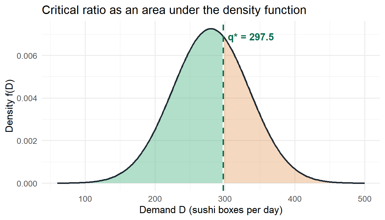
With $CR = 0.625$ we obtain $z^* = \Phi^{-1}(0.625) \approx 0.319$ and thus $q^* = 280 + 55 \cdot 0.319 \approx 297.5$ sushi boxes. Since only whole boxes can be produced, in practice one would round up to $q^* = 298$. The expected shortage and overstock costs at the optimum amount to around €166.8 per day, so that the expected profit is $E[P(q^*)] = \mu \cdot c^u - E[C(q^*)] \approx 280 \cdot 5 - 166.8 \approx 1{,}233.2\,$€ per day.
As a check, we compare our own result directly with the ready-made function from `R/scm_functions.R`:
```{r ch7-vergleich-funktion}
source("../R/scm_functions.R")

ergebnis_fertig <- newsvendor_normal(
  mu = mu_nachfrage, sigma = sigma_nachfrage,
  p = 10, c = 5, s = 2
)

ergebnis_fertig$q_star       # should match q_stern_normal
ergebnis_fertig$exp_profit # expected profit at the optimum
```
The following figure illustrates the demand distribution together with the optimal order quantity: the green shaded area to the left of $q^*$ corresponds to the cumulative probability $F(q^*) = CR$, i.e. the proportion of days on which the order quantity is sufficient.
```{r}
#| label: fig-newsvendor-normal
#| fig-cap: "Density of the normally distributed sushi demand of the Frankfurt store with optimal order quantity"
#| fig-width: 7
#| fig-height: 4
nachfrage_grid <- tibble(
  d      = seq(mu_nachfrage - 4 * sigma_nachfrage,
               mu_nachfrage + 4 * sigma_nachfrage,
               length.out = 300),
  dichte = dnorm(d, mean = mu_nachfrage, sd = sigma_nachfrage)
)

ggplot(nachfrage_grid, aes(x = d, y = dichte)) +
  geom_area(
    data = filter(nachfrage_grid, d <= q_stern_normal),
    fill = "#52B788", alpha = 0.45
  ) +
  geom_area(
    data = filter(nachfrage_grid, d >= q_stern_normal),
    fill = "#D97B29", alpha = 0.30
  ) +
  geom_line(linewidth = 1, colour = "#1F2933") +
  geom_vline(
    xintercept = q_stern_normal,
    linetype = "dashed", colour = "#0B6E4F", linewidth = 1
  ) +
  annotate(
    "text", x = q_stern_normal, y = max(nachfrage_grid$dichte) * 0.95,
    label = paste0("q* = ", round(q_stern_normal, 1)),
    hjust = -0.1, colour = "#0B6E4F", fontface = "bold"
  ) +
  labs(
    x = "Demand D (sushi boxes per day)",
    y = "Density f(D)",
    title = "Critical ratio as an area under the density function"
  ) +
  theme_minimal(base_size = 13)
```
A methodological digression is permitted at this point: instead of using the formula for $q^*$ directly, the expected profit $E[P(q)]$ could also be determined approximately by **Monte Carlo simulation** — exactly as introduced in Chapter [-@sec-unsicherheit-pooling]. One would draw a very large number of random daily demands with `rnorm()`, compute the realised profit for each draw according to the profit function $P(D,q)$ and then average over all replications (for instance with `replicate()`). For a sufficiently large number of simulation runs, this simulated mean converges to the expected value $E[P(q)]$ calculated analytically here — a good plausibility test when a closed-form formula is available, as here, and the only practicable solution when it is not.
### Three cases using the Frankfurt store as an example
The distinction of cases from the discrete section can be quantified directly for the Frankfurt store. To this end, the lecture varies the cost rates so that underage is cheaper than, equally expensive as or more expensive than overage:
```{r}
#| label: ch7-drei-faelle
faelle <- tibble(
  Case = c("1: c^u < c^o", "2: c^u = c^o", "3: c^u > c^o"),
  cu   = c(1, 3, 5),
  co   = c(5, 3, 1)
) |>
  mutate(
    CR      = cu / (cu + co),
    z_stern = qnorm(CR),
    q_stern = mu_nachfrage + sigma_nachfrage * z_stern,
    E_Cost = (cu + co) * sigma_nachfrage * dnorm(z_stern)
  )

faelle |> mutate(across(where(is.numeric), ~ round(.x, 2)))
```
In the first case (overstocks five times as expensive as shortages), SushiFresh produces around `r round(faelle$q_stern[1])` boxes, clearly **below** the expected value of 280 boxes, and deliberately accepts that the goods will be sold out before closing time on around `r round((1-faelle$CR[1])*100)`% of days. In the symmetric case, the median – identical to the mean for the normal distribution – is optimal. In the third case, around `r round(faelle$q_stern[3])` boxes are produced, clearly **above** the expected value. Because of the symmetry of the normal distribution, cases 1 and 3 lie as mirror images around $\mu$. It is noteworthy that the minimum expected costs in cases 1 and 3 are equally high: they depend only on $c^u + c^o$ and $\varphi(z^*)$, and $\varphi$ is symmetric.
## Numerical optimisation as an alternative to the closed-form solution
For the normal distribution we were able to determine $q^*$ conveniently via `qnorm()` because its distribution function has a known inverse. For many practically relevant distributions — for instance a lognormal, gamma or empirically estimated distribution — no closed form exists for $F^{-1}$. In such cases numerical **optimisation** helps, as introduced in the following aside.
::: {.r-exkurs}
**R aside: `uniroot()` and `optimize()` instead of an analytical solution**
The condition $F(q^*) = CR$ from the fractile rule can be viewed as a **root-finding problem**: we are looking for the value $q$ for which the function $g(q) = F(q) - CR$ becomes zero. The function `uniroot()` finds exactly such a root within a given interval — without us having to know the inverse function of $F$ explicitly:
```{r ch7-uniroot}
# Objective function: difference between distribution function and critical ratio.
# On success, uniroot() returns the q for which this difference becomes zero.
zielfunktion_wurzel <- function(q) {
  pnorm(q, mean = mu_nachfrage, sd = sigma_nachfrage) - cr
}

loesung_uniroot <- uniroot(
  zielfunktion_wurzel,
  interval = c(mu_nachfrage - 4 * sigma_nachfrage,
               mu_nachfrage + 4 * sigma_nachfrage)
)

loesung_uniroot$root   # should (almost) match q_stern_normal
```
Alternatively, the expected cost function $E[C(q)]$ can also be **minimised directly** without the detour via the fractile rule — useful, for instance, when only the cost function is known but not its analytical minimum. `integrate()` computes the expected values $E[(D-q)^+]$ and $E[(q-D)^+]$ numerically, and `optimize()` then searches for the minimum of the total cost function:
```{r ch7-optimize}
erwartete_kosten <- function(q) {
  e_fehlmenge <- integrate(
    function(d) (d - q) * dnorm(d, mean = mu_nachfrage, sd = sigma_nachfrage),
    lower = q, upper = mu_nachfrage + 8 * sigma_nachfrage
  )$value

  e_ueberbestand <- integrate(
    function(d) (q - d) * dnorm(d, mean = mu_nachfrage, sd = sigma_nachfrage),
    lower = mu_nachfrage - 8 * sigma_nachfrage, upper = q
  )$value

  cu * e_fehlmenge + co * e_ueberbestand
}

loesung_optimize <- optimize(
  erwartete_kosten,
  interval = c(mu_nachfrage - 4 * sigma_nachfrage,
               mu_nachfrage + 4 * sigma_nachfrage)
)

loesung_optimize$minimum   # optimal order quantity
loesung_optimize$objective # minimum expected costs
```
Both numerical methods yield (apart from minimal rounding deviations) the same result as the closed-form formula $q^* = \mu + \sigma \cdot \Phi^{-1}(CR)$. The advantage of this approach becomes apparent as soon as `dnorm()`/`pnorm()` are replaced by the density or distribution function of any other distribution — the structure of the code remains unchanged, whereas an analytical derivation would have to be carried out anew for each new distribution.
:::
## Critical ratio and service level
The critical ratio $CR = \Phi(z^*)$ has a second, very practical interpretation: it corresponds exactly to the probability that demand does **not** exceed the order quantity, i.e. the so-called **cycle service level** ($\alpha$ service level) — the proportion of periods in which the entire demand can be met from the available quantity. For our example, $CR = 0.625$ means: on about 62.5% of all days the order quantity $q^*$ is sufficient to serve the complete daily demand; on the remaining roughly 37.5% of days a (partial) shortage occurs.
This relationship is the reason why the newsvendor model is important far beyond single-period problems (the lecture emphasises: it is the basis for calculating cost-optimal safety stocks in inventory systems; in Chapter [-@sec-bullwhip] the order-up-to level $S = \mu(l+1) + z_{CR}\,\sigma\sqrt{l+1}$ is derived from it): in practice, the **safety stocks** of multi-period inventory systems are very often dimensioned according to exactly this principle — a desired service level is set (e.g. 95%) and the required safety factor is determined from it via $z = \Phi^{-1}(\text{service level})$, as already hinted at in Chapter [-@sec-unsicherheit-pooling] in the context of the pooling effect. The only difference from the newsvendor model lies in *where* the target value of the critical ratio comes from: in the newsvendor model it is derived from costs ($CR = c^u/(c^u+c^o)$), whereas in many operational inventory systems it is frequently specified directly as a management decision. It should also be noted that the cycle service level considered here (probability of *no* shortage) must not be confused with the **fill rate**, which measures the proportion of demand met *in terms of quantity* and is as a rule higher than the cycle service level.
## Sensitivity analysis: how does the model respond to changed parameters?
So far we have solved the newsvendor model for fixed values of $\mu$, $\sigma$, $p$, $c$ and $v$. In practice, one is often interested in **how sensitively** the optimal decision reacts to changes in these parameters — for instance when the selling price fluctuates seasonally or the demand estimate is subject to uncertainty. **Vectorisation**, which you already know from Chapter [-@sec-standort-1] (`sapply()`) and Chapter [-@sec-standort-2] (`purrr::map()`), is ideal for exactly this: instead of evaluating the model for a single parameter value, we apply it to a whole vector of possible values.
::: {.r-exkurs}
**R aside: sensitivity analysis through vectorisation**
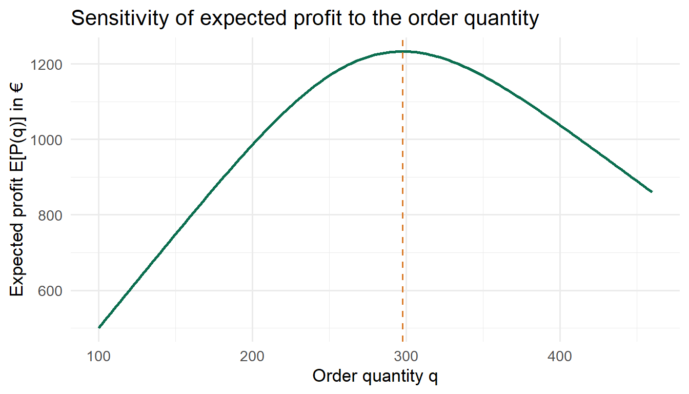
First, we examine how the expected profit $E[P(q)]$ behaves over a fine grid of possible order quantities — for the Frankfurt store, i.e. for every quantity between 100 and 460 boxes. To do so, we encapsulate the profit formula from the normal distribution case in a small function and evaluate it with `sapply()` for each grid point:
```{r}
#| label: fig-newsvendor-sensitivitaet-q
#| fig-cap: "Expected profit as a function of the order quantity q"
#| fig-width: 7
#| fig-height: 4
# Model function: expected profit for a given q (normal distribution case)
erwarteter_gewinn_normal <- function(q, mu, sigma, cu, co) {
  z <- (q - mu) / sigma
  L <- function(z) dnorm(z) - z * (1 - pnorm(z))  # standard normal loss function
  e_fehlmenge    <- sigma * L(z)
  e_ueberbestand <- sigma * L(-z)
  mu * cu - cu * e_fehlmenge - co * e_ueberbestand
}

q_raster <- seq(100, 460, by = 2)

# sapply() applies the function to each value of the grid
gewinn_je_q <- sapply(
  q_raster, erwarteter_gewinn_normal,
  mu = mu_nachfrage, sigma = sigma_nachfrage, cu = cu, co = co
)

sensitivitaet_q <- tibble(bestellmenge = q_raster, erwarteter_gewinn = gewinn_je_q)

ggplot(sensitivitaet_q, aes(x = bestellmenge, y = erwarteter_gewinn)) +
  geom_line(colour = "#0B6E4F", linewidth = 1) +
  geom_vline(xintercept = q_stern_normal, linetype = "dashed", colour = "#D97B29") +
  labs(
    x = "Order quantity q", y = "Expected profit E[P(q)] in €",
    title = "Sensitivity of expected profit to the order quantity"
  ) +
  theme_minimal(base_size = 13)
```
The curve vividly confirms what we had already derived analytically: the expected profit is a **concave** function of the order quantity with a unique maximum at $q^*$ — both significantly smaller and significantly larger quantities reduce the expected profit.
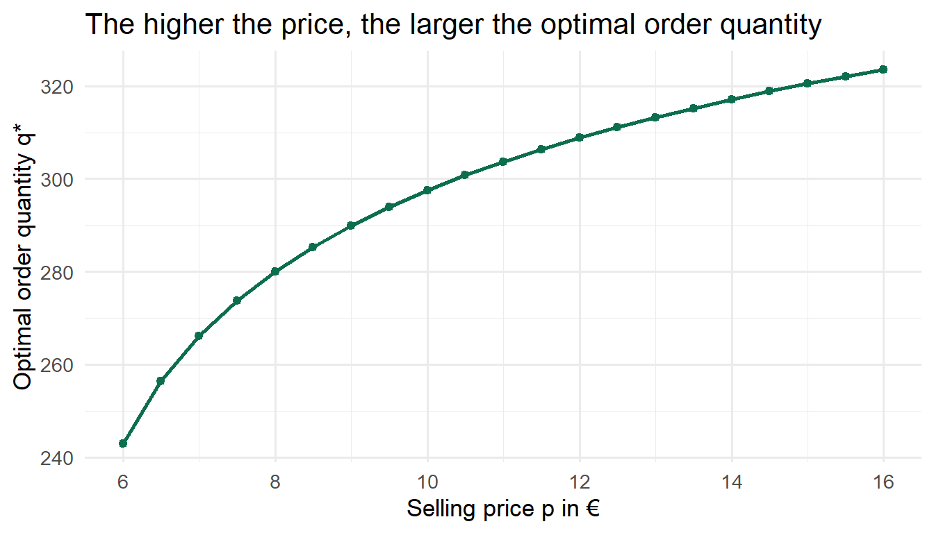
In a second step, we examine how much the *optimal* order quantity itself changes when the selling price $p$ changes (e.g. due to seasonal discount promotions). For this we use `purrr::map_dbl()`, which — analogous to `sapply()` — iterates a function over a vector and is guaranteed to return a numeric vector:
```{r}
#| label: fig-newsvendor-sensitivitaet-preis
#| fig-cap: "Optimal order quantity as a function of the selling price"
#| fig-width: 7
#| fig-height: 4
herstellkosten <- 5   # remains constant
restwert       <- 2   # remains constant
preise         <- seq(6, 16, by = 0.5)

q_stern_je_preis <- purrr::map_dbl(preise, function(p) {
  cu_tmp <- p - herstellkosten          # underage cost changes with p
  cr_tmp <- cu_tmp / (cu_tmp + co)      # co remains unchanged
  mu_nachfrage + sigma_nachfrage * qnorm(cr_tmp)
})

sensitivitaet_preis <- tibble(preis = preise, q_stern = q_stern_je_preis)

ggplot(sensitivitaet_preis, aes(x = preis, y = q_stern)) +
  geom_line(colour = "#0B6E4F", linewidth = 1) +
  geom_point(colour = "#0B6E4F") +
  labs(
    x = "Selling price p in €", y = "Optimal order quantity q*",
    title = "The higher the price, the larger the optimal order quantity"
  ) +
  theme_minimal(base_size = 13)
```
The graph shows an intuitive relationship: if the selling price $p$ rises, the underage cost $c^u = p - c$ rises and thus also the critical ratio $CR$ — the supplier should therefore tend to order **more**, because a shortage has now become more expensive. In practice, such sensitivity analyses are often at least as valuable as the single optimal value itself, because they show how robust a decision is to estimation errors or market fluctuations.
:::
## Areas of application and limitations of the model
The newsvendor model is most useful where **smoothing demand through inventory holding is not possible** and the cost parameters $c^u$ and $c^o$ can be estimated sufficiently well [@thonemann2023operations]. Typical areas of application are:
- **Seasonal and promotional items** (Christmas items, fashion goods for one season), for which reordering within the season is practically ruled out,
- **Fresh goods with a short shelf life** (like our sushi example, but also bakery products, flowers or ready meals),
- **Tickets for events or means of transport**, whose capacity is fixed on the day of the event or departure,
- **Capacity planning** in manufacturing, when capacity can only be set once before the start of a period.
Beyond this, the newsvendor model — as shown in the previous section — is the conceptual basis for calculating cost-optimal safety stocks in multi-period inventory systems, which raises its practical importance far beyond the individual case of a one-off order decision [@silver2017inventory].
Nevertheless, the model rests on a number of assumptions that need to be examined critically in practice: it is assumed that the demand distribution is **known and stationary**, that the decision-maker is **risk-neutral** (i.e. maximises only the *expected* profit without taking risk aversion towards losses into account), that no **fixed ordering costs** are incurred and that **one** order decision actually covers the entire period. Substitution effects between similar products, learning effects from repeated decisions or the interplay with upstream and downstream stages of the supply chain — topics we will encounter again in the next chapter on the bullwhip effect — are not considered in the basic model and may require extensions [@cachon2024matching; @chopra2025supply].
## Summary
The newsvendor model answers the question of the optimal order quantity for a one-off decision under uncertain demand. The starting point is the underage cost $c^u = p - c$ and the overage cost $c^o = c - v$, whose ratio yields the critical ratio $CR = c^u/(c^u+c^o)$. This corresponds both to the quantile of the demand distribution that determines the optimal order quantity ($q^* = F^{-1}(CR)$) and to the economically sensible service level. With discrete demand, the smallest quantity whose cumulative probability reaches at least $CR$ is chosen; with normally distributed demand, $q^*$ can be calculated directly via $\mu + \sigma \cdot \Phi^{-1}(CR)$. Methodologically, you have learned to encapsulate a complete decision model in your own R function, to search numerically for optimal solutions with `uniroot()` and `optimize()` when no closed-form formula is available, and to carry out and visualise sensitivity analyses with vectorised model calls (`sapply()`, `purrr::map_dbl()`). These three techniques — custom model functions, numerical optimisation and vectorised sensitivity analyses — will come up again and again in the following chapters.
::: {.kontrollfragen}
**Review questions**
1. Name the four characteristic features that make a decision situation a newsvendor problem. Why is the sushi example so well suited to this?
2. Define the underage and overage costs $c^u$ and $c^o$ in your own words using the sushi example. Why are these opportunity costs and not actual cash outflows?
3. Derive the critical ratio $CR = c^u/(c^u+c^o)$ using a marginal analysis (what happens if the order quantity is increased marginally by one unit?).
4. A magazine retailer buys copies for €2, sells them for €5 and can return unsold copies to the publisher for €0.50. Daily demand follows the scenarios $\{20, 30, 40\}$ with probabilities $\{0.3;\ 0.5;\ 0.2\}$. Determine $c^u$, $c^o$, $CR$ and the optimal order quantity.
5. Why does the fractile rule with discrete demand usually not yield an exact equality $F(q^*)=CR$, whereas it does with continuous demand? Which decision rule applies in the discrete case?
6. Explain the relationship between the critical ratio and the cycle service level. How does the cycle service level differ from the fill rate?
7. In which situations would you prefer `uniroot()` or `optimize()` to an analytical solution formula such as $q^* = \mu + \sigma \cdot \Phi^{-1}(CR)$? Give an example of a demand distribution for which this makes sense.
8. Name three typical areas of application of the newsvendor model as well as two central assumptions that need to be questioned critically in practice.
:::