9  The Bullwhip Effect and the Beer Game

Learning objectives

• define the bullwhip effect and explain it using a running example
• apply the inventory measures of a multi-echelon supply chain (on-hand inventory, net inventory, inventory position) to a concrete ordering situation
• calculate and interpret the variance ratio as a measure of the bullwhip effect
• distinguish the four classic causes of the bullwhip effect and assign examples to them
• classify the Beer Game as a didactic simulation game and reproduce it with your own R simulation
• understand time series in R as vectors and analyse them with diff() and dplyr::lag()
• model a multi-echelon supply chain in your own simulation loop in R and visualise it with facets
• assess countermeasures against the bullwhip effect (information sharing, VMI, CPFR, shorter replenishment lead times)

9.1 From the single stage to the chain

In the preceding chapters we always considered uncertainty from the perspective of a single stage of a supply chain: a retailer or producer knows (approximately) the distribution of demand, derives a safety stock from it and sets an order-up-to level that achieves a desired service level. The pooling principle and the newsvendor model thus answer the question: How much should a stage keep in stock when it is confronted with uncertain demand?

In reality, however, practically every stage of a supply chain is simultaneously the customer of an upstream stage and the supplier of a downstream stage. The “demand” a wholesaler has to deal with is not the demand of end consumers but the order quantity of the retailer – and this order quantity is itself already the result of an inventory decision based on an estimated, uncertain demand. Each stage thus filters, interprets and amplifies the information it passes on to the next stage. Precisely this phenomenon of the stage-by-stage amplification of demand fluctuations along a supply chain is the subject of this – final – chapter: the bullwhip effect (occasionally also called the Peitscheneffekt, “whip effect”, in German).

As usual, we approach the topic through a running case example, derive a formal definition and a measurement concept from it, classify the causes and consequences of the effect and get to know the Beer Game, a classic teaching game that we then rebuild ourselves in R. At the end there is an overview of countermeasures used in practice to “defuse” the whip.

9.2 Case example: the SushiFresh supply chain

We return once more to SushiFresh GmbH from the previous chapters: the regional producer of fresh sushi boxes with a central kitchen in Raunheim (cf. the location analysis in Chapter 6 and the pooling arguments in Chapter 7), which supplies six supermarket stores in the Rhine-Main area – among them the particularly high-demand Frankfurt store already familiar from Chapters 7 and 8 (\(\mu=280\), \(\sigma=55\) sushi boxes per day). For production, SushiFresh depends on the daily delivery of fresh fish fillets supplied by the fish wholesaler Nord-Fisch KG. Nord-Fisch procures raw fish, produces fillets from it and stores them in order to be able to deliver quickly. The chain thus has three stages; orders flow upstream, deliveries downstream:

\[ \text{Supermarket stores} \;\longleftrightarrow\; \text{SushiFresh GmbH} \;\longleftrightarrow\; \text{Nord-Fisch KG} \]

The stores observe end-customer demand (e.g. Frankfurt: \(\mu=280\), \(\sigma=55\)) and order sushi boxes from SushiFresh every day. SushiFresh receives these orders as its demand, orders fish from Nord-Fisch and holds a stock of fish fillets. Nord-Fisch in turn sees only the orders from SushiFresh. SushiFresh and Nord-Fisch both hold a (safety) stock of fish fillets to avoid shortages – so the central question is: How high should this stock be, and how do the ordering decisions affect the upstream stage?

Each stage observes only the orders of the stage immediately downstream of it and must derive its own ordering decision from these – without insight into actual end-customer demand. To be able to capture this decision formally, we need three inventory measures that are updated in every period \(t\):

• the on-hand inventory \(i_t\): the quantity actually available in the warehouse, \(i_t = \max(0,\, i_{t-1} + q_{t-l} - d_t)\)
• the net inventory \(n_t\): on-hand inventory minus open shortages (backorders), \(n_t = i_{t-1} + q_{t-l} - d_t\)
• the inventory position \(p_t\): net inventory plus all orders already placed but not yet received (the so-called pipeline), \(p_t = n_t + \sum_{\tau=t-l+1}^{t-1} q_\tau\)

Here \(d_t\) denotes the demand in period \(t\), \(q_t\) the order quantity and \(l\) the replenishment lead time in periods. If a stage sets an order-up-to level \(S\), the order quantity results from topping up the inventory position to \(S\):

\[ q_t = \max\bigl(0,\; S - p_t\bigr) \]

The order-up-to level itself is composed – as derived in the chapter on the newsvendor model – of a base demand over the protection period \(l+1\) (the time from one ordering decision until the next possible reaction to a new delivery) and a safety stock:

\[ S = \mu \cdot (l+1) + z_\alpha \cdot \sigma \cdot \sqrt{l+1} \]

Here \(\mu\) and \(\sigma\) are the expected demand per period and its standard deviation, which in practice have to be estimated from past demand, and \(z_\alpha\) is the quantile of the standard normal distribution for the desired service level \(\alpha\).

It is precisely this estimation that the bullwhip effect hinges on. If we simulate SushiFresh GmbH for twelve days with the moderately fluctuating sushi box demand of the Frankfurt store (\(\mu=280\), \(\sigma=55\)), a replenishment lead time of two days (one day of lead time for the fish delivery by Nord-Fisch KG, another day for production and delivery to the store) and an – initially fixed – order-up-to level of \(S=990\), we can use the function simuliere_tS() from R/scm_functions.R, which automates this updating of on-hand inventory, net inventory and inventory position:

# Observed sushi box demand of the Frankfurt store (units per day,
# mu = 280, sigma = 55 - cf. newsvendor and pooling chapters)
nachfrage <- c(234, 256, 344, 410, 278, 322, 212, 256, 278, 234, 256, 278)

# Simulation of a (t,S) inventory policy at SushiFresh GmbH: daily
# ordering decision (t=1), fixed order-up-to level S = 990,
# initial inventory 990, replenishment lead time 2 days
sushi_sim <- simuliere_tS(
  bedarf         = nachfrage,
  t              = 1,
  S              = 990,
  anfangsbestand = 990,
  wbz            = 2
)

sushi_sim |>
  select(Periode, Bedarf, Nettobestand, Disponibler_Bestand_vor_Bestellung, Bestellmenge) |>
  kable(digits = 1, align = "r",
        col.names = c("Period", "Demand", "Net inventory",
                      "Inventory position before order", "Order quantity"),
        caption = "Simulated inventory and order development of SushiFresh GmbH (Frankfurt store)")

Simulated inventory and order development of SushiFresh GmbH (Frankfurt store)

Period	Demand	Net inventory	Inventory position before order	Order quantity
1	234	756	756	234
2	256	500	734	256
3	344	390	646	344
4	410	236	580	410
5	278	302	712	278
6	322	390	668	322
7	212	456	778	212
8	256	522	734	256
9	278	456	712	278
10	234	478	756	234
11	256	500	734	256
12	278	456	712	278

Although the order-up-to level \(S=990\) remains constant over all twelve days, the order quantity follows the course of demand exactly, merely shifted by the replenishment lead time: because there are two days between order and delivery, every deviation in demand affects the inventory position – and thus the next order – only with a delay, but in full. We can read this relationship directly from the standard deviations:

sd_nachfrage  <- sd(sushi_sim$Bedarf)
sd_bestellung <- sd(sushi_sim$Bestellmenge)

tibble(
  Measure              = c("Demand d[t]", "Order quantity q[t]"),
  `Standard deviation` = round(c(sd_nachfrage, sd_bestellung), 2)
) |>
  kable(align = "lr")

Measure	Standard deviation
Demand d[t]	55.07
Order quantity q[t]	55.07

Definition: bullwhip effect

The bullwhip effect (also whip effect or Forrester effect) is present when the variability of the orders of one stage of a supply chain is greater than the variability of the demand this stage faces – and this amplification continues or intensifies with each further upstream stage (Cachon and Terwiesch 2024). Formally, the following often holds:

\[ \operatorname{Var}(d_t) \;<\; \operatorname{Var}\!\bigl(q_t^{\,i}\bigr) \;<\; \operatorname{Var}\!\bigl(q_t^{\,i+1}\bigr) \;<\; \operatorname{Var}\!\bigl(q_t^{\,i+2}\bigr) \;<\; \dots \]

where \(q_t^{\,i}\) denotes the order quantity of the \(i\)-th stage (counted from the end customers) in period \(t\).

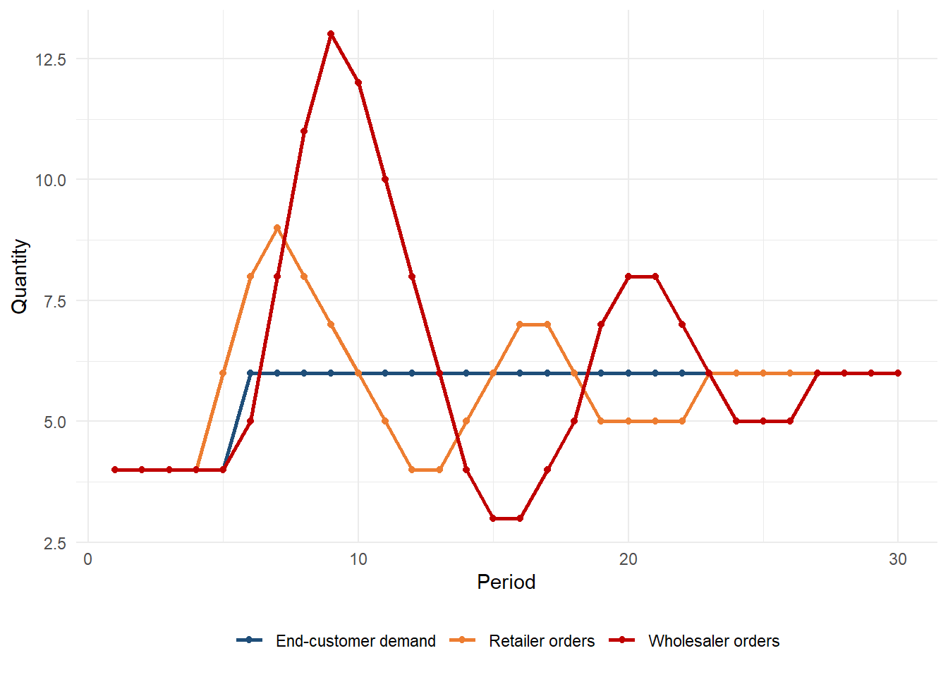
The lecture quotes the original definition by Cachon and Terwiesch (2024): “The bullwhip effect is present in a supply chain if the variability of demand at one level of the supply chain is greater than the variability of demand at the next downstream level in the supply chain, where variability is measured with the coefficient of variation.” The addition regarding the coefficient of variation \(CV = \sigma/\mu\) is important: it makes stages comparable that work in different units or orders of magnitude (e.g. sushi boxes at the store, kilograms of fish at the wholesaler). The typical patterns are shown in the following schematic figure: end-customer demand rises once from 4 to 6 units; retail orders overshoot in response, wholesale orders even more strongly and for longer, before all stages settle at the new level.

verlauf <- tibble(
  Periode = 1:30,
  `End-customer demand` = c(rep(4, 5), rep(6, 25)),
  `Retailer orders` = c(rep(4, 4), 6, 8, 9, 8, 7, 6, 5, 4, 4, 5, 6, 7, 7, 6,
                                5, 5, 5, 5, 6, 6, 6, 6, 6, 6, 6, 6),
  `Wholesaler orders` = c(rep(4, 5), 5, 8, 11, 13, 12, 10, 8, 6, 4, 3, 3, 4, 5,
                              7, 8, 8, 7, 6, 5, 5, 5, 6, 6, 6, 6)
) |>
  pivot_longer(-Periode, names_to = "Reihe", values_to = "Menge")

ggplot(verlauf, aes(Periode, Menge, colour = Reihe)) +
  geom_line(linewidth = 1) + geom_point(size = 1.5) +
  scale_colour_manual(values = c("End-customer demand" = "#1F4E79",
                                 "Retailer orders" = "#ED7D31",
                                 "Wholesaler orders" = "#C00000")) +
  labs(x = "Period", y = "Quantity", colour = NULL) +
  theme_minimal() + theme(legend.position = "bottom")

Schematic pattern: amplification of a one-off demand step across two stages

The consequences upstream are an “escalation” of order quantities, increasing volatility of inventories and more frequent shortages – although end-customer demand has changed only once and only moderately.

The reason for this amplification already lies in the structure of the ordering rule: the order quantity \(q_t = S - p_t\) is made up of several components that are not reflected one-to-one in actual demand,

\[ q_t = \underbrace{\hat{\mu}\cdot(l+1)}_{\text{expected demand}} \;+\; \underbrace{(n_{t-1}^{\text{target}} - n_{t-1})}_{\text{inventory correction}} \;+\; \underbrace{z_\alpha\,\hat\sigma\sqrt{l+1}}_{\text{safety stock correction}}, \]

and for an upstream stage it is not apparent whether a higher order quantity indicates a lasting shift in end-customer demand or is merely a short-term inventory correction. This ambiguity makes the upstream stage’s own forecast more difficult – its forecast error \(\hat\sigma\) rises, and with it (via the term above) its own order quantity variance. The effect thus propagates from stage to stage and typically becomes larger the further one moves away from the end customers.

9.3 R aside: time series as vectors and the function diff()

R aside: time series and diff()

A time series is initially nothing special in R: a simple numeric vector whose order corresponds to the chronological sequence of the observations. The vector nachfrage from the sushi box example contains twelve values for twelve days – R initially needs nothing more to work with a time series.

A very common question with time series is: How much does the quantity change from one period to the next? For this, R offers the function diff(), which for a vector x of length \(n\) returns a new vector of length \(n-1\) whose \(t\)-th element is \(x_{t+1} - x_t\):

# diff() calculates the change from one period to the next:
# diff(x)[t] = x[t+1] - x[t]
veraenderung_nachfrage <- diff(nachfrage)
veraenderung_nachfrage

 [1]   22   88   66 -132   44 -110   44   22  -44   22   22

# one value fewer than in the original vector, since no previous-period
# value exists for period 1
length(nachfrage)

[1] 12

length(veraenderung_nachfrage)

[1] 11

# mean absolute change as a simple measure of volatility:
# comparing this for demand and order quantity in the first,
# simple case example with constant S
mean(abs(diff(nachfrage)))

[1] 56

mean(abs(diff(sushi_sim$Bestellmenge)))

[1] 56

The mean absolute period-to-period change of order quantity and demand is identical in this first, simple case example – not a coincidence but a direct consequence of the ordering rule: with daily review (\(t=1\)) and a constant order-up-to level \(S\), exactly \(q_t = d_t\) holds (only delivered with a delay of the replenishment lead time), because each order tops the inventory position back up by exactly the amount consumed in the previous period. Amplification only arises as soon as the order-up-to level itself – as is usual in practice – is recalculated from rolling estimates of the demand parameters; this is exactly what we reproduce further below in the multi-echelon simulation. diff() can also be extended with the argument lag to larger time intervals (diff(x, lag = 2)) or with differences to repeated differencing – but we will not go into this further here.

9.4 Measuring the bullwhip effect: the variance ratio

In order not only to describe the bullwhip effect qualitatively but to quantify it, the literature mostly uses the variance ratio (bullwhip ratio):

\[ B \;=\; \frac{\operatorname{Var}(q_t)}{\operatorname{Var}(d_t)} \qquad \text{or stage by stage} \qquad B^{\,i} \;=\; \frac{\operatorname{Var}\!\bigl(q_t^{\,i}\bigr)}{\operatorname{Var}\!\bigl(q_t^{\,i-1}\bigr)}. \]

If \(B>1\), a stage amplifies the variance of the demand it faces; \(B=1\) means that the order variance corresponds exactly to the demand variance (no bullwhip effect); \(B<1\) would even indicate smoothing. In the original definition, the coefficient of variation (\(\text{CV}=\sigma/\mu\)) is often used instead of the pure variance in order to compensate for scale effects between the stages; for practical application, however – especially when \(\mu\) remains similar across the stages – the simple variance ratio is the more common and easier-to-calculate metric.

For our sushi box example, \(B\) can be calculated with a single line of R code:

bullwhip_mass_sushi <- var(sushi_sim$Bestellmenge) / var(sushi_sim$Bedarf)
round(bullwhip_mass_sushi, 2)

[1] 1

In this first, deliberately simple case example, \(B=1.00\) – SushiFresh GmbH does not yet amplify the demand fluctuation of the Frankfurt store here. This is not an error but follows necessarily from the ordering rule: as long as the order-up-to level \(S\) remains constant and is reviewed daily, the order quantity corresponds exactly to the (time-shifted) demand – the order-up-to rule merely passes demand on unchanged. The bullwhip effect only arises when \(S\) itself is periodically recalculated from rolling estimated demand parameters \(\hat\mu\) and \(\hat\sigma\), as is the case in practice – and in the following section on multi-echelon simulation: there the order quantity of one stage becomes the (distorted) “demand” of the next stage, and with each re-estimation of \(\hat\mu\) and \(\hat\sigma\) the order variance continues to grow, although each stage strictly follows the same simple, rational order-up-to rule. The bullwhip effect is therefore not a sign of irrational behaviour by individuals but a structural property of the interaction of rolling forecasts, inventory policy and replenishment lead time.

9.5 Rolling parameter estimation: how the bullwhip effect arises

In practice, SushiFresh does not know the parameters \(\mu\) and \(\sigma\) but continually estimates them from the most recently observed demand – for instance with a moving average and the empirical standard deviation over the last \(T\) days: \[ \hat{\mu}_t = \frac{1}{T} \sum_{\tau=t-T}^{t-1} d_\tau, \qquad \hat{\sigma}_t = \sqrt{\frac{1}{T-1} \sum_{\tau=t-T}^{t-1} \big(d_\tau - \hat{\mu}_t\big)^2 } . \] \(\hat\sigma_t\) measures the dispersion of demand around the forecast and thus the forecast error. With these estimates, the order-up-to level is recalculated every day: \(S_t = (l+1)\,\hat\mu_t + z_\alpha\,\hat\sigma_t\sqrt{l+1}\). The lecture works through this procedure for the same twelve days, with an estimation window of \(T = 3\) days, \(l = 2\) and \(\alpha = 95\%\):

fenster     <- 3
wbz_s       <- 2
z_95        <- qnorm(0.95)
n_t         <- length(nachfrage)

mu_hat <- sigma_hat <- S_t <- numeric(n_t)
bestellung_dyn <- lieferung_dyn <- netto_dyn <- dispo_dyn <- numeric(n_t)
netto_vor <- 990                               # initial inventory

for (t in seq_len(n_t)) {
  # 1. parameter estimation from the (at most) 'fenster' previous days;
  #    on the first day: planning values of the Frankfurt store (280 / 55)
  hist <- if (t == 1) numeric(0) else nachfrage[max(1, t - fenster):(t - 1)]
  mu_hat[t]    <- if (length(hist) == 0) 280 else mean(hist)
  sigma_hat[t] <- if (length(hist) < 2) 55 else sd(hist)
  S_t[t]       <- (wbz_s + 1) * mu_hat[t] + z_95 * sigma_hat[t] * sqrt(wbz_s + 1)

  # 2. delivery of the order placed wbz days ago arrives, demand occurs
  lieferung_dyn[t] <- if (t > wbz_s) bestellung_dyn[t - wbz_s] else 0
  netto_dyn[t]     <- netto_vor + lieferung_dyn[t] - nachfrage[t]

  # 3. inventory position = net inventory + outstanding orders
  offen <- if (t == 1) 0 else sum(bestellung_dyn[max(1, t - wbz_s + 1):(t - 1)])
  dispo_dyn[t] <- netto_dyn[t] + offen

  # 4. top up to the (newly estimated) order-up-to level
  bestellung_dyn[t] <- max(0, S_t[t] - dispo_dyn[t])
  netto_vor <- netto_dyn[t]
}

tibble(Day = 1:n_t, Demand = nachfrage, mu_hat = mu_hat, sigma_hat = sigma_hat,
       S_t = S_t, Order = bestellung_dyn) |>
  kable(digits = 1, caption = "Ordering decisions with rolling parameter estimation")

Ordering decisions with rolling parameter estimation

Day	Demand	mu_hat	sigma_hat	S_t	Order
1	234	280.0	55.0	996.7	240.7
2	256	234.0	55.0	858.7	118.0
3	344	245.0	15.6	779.3	264.6
4	410	278.0	58.2	999.8	630.5
5	278	336.7	77.3	1230.1	508.3
6	322	344.0	66.0	1220.0	311.9
7	212	336.7	67.2	1201.5	193.5
8	256	270.7	55.4	969.7	24.3
9	278	263.3	55.4	947.7	256.0
10	234	248.7	33.6	841.7	128.0
11	256	256.0	22.0	830.7	244.9
12	278	256.0	22.0	830.7	278.0

c(sd_demand  = sd(nachfrage),
  sd_order   = sd(bestellung_dyn),
  B          = var(bestellung_dyn) / var(nachfrage))

 sd_demand   sd_order          B 
 55.066626 165.049878   8.983663 

The standard deviation of the order quantities, at around 165 boxes, is now considerably larger than that of demand (55 boxes); the variance ratio is \(B \approx 9\). SushiFresh thus creates additional uncertainty for Nord-Fisch, although nothing has changed in end-customer demand. The cause can be clearly seen on days 4 and 5: the high demand on days 3 and 4 (344 and 410 boxes) enters the estimation window and increases \(\hat\mu_t\) – and each increase in \(\hat\mu_t\) acts on the order-up-to level with the multiplier \((l+1) = 3\), which rises by more than 400 boxes within two days. At the same time \(\hat\sigma_t\) rises because the forecast error grows. SushiFresh therefore not only reorders the additional consumption but also builds up additional stock – and reduces its orders all the more sharply as soon as the high values have left the estimation window again.

In depth (theory): a lower bound for the bullwhip effect

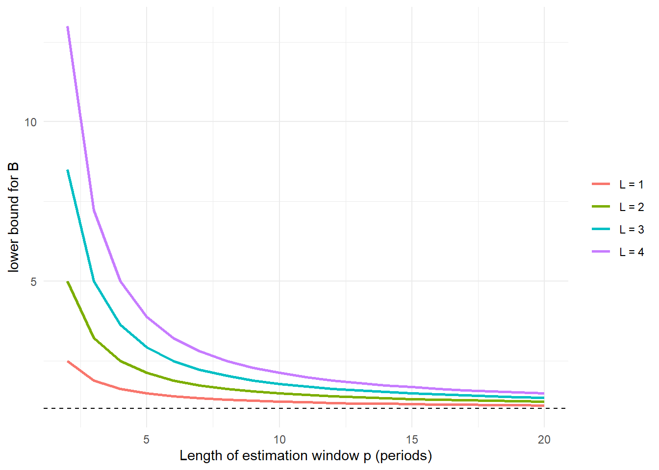
Chen et al. (2000) analysed the mechanism visible in the table analytically. They consider a stage that orders according to an order-up-to policy, has the replenishment lead time \(L\) and estimates mean demand with a moving average over the last \(p\) periods. For independent, identically distributed demand, they show that the variance ratio is at least \[ B = \frac{\operatorname{Var}(q)}{\operatorname{Var}(d)} \;\geq\; 1 + \frac{2L}{p} + \frac{2L^2}{p^2} \] (The bound holds when the standard deviation is also estimated; if only the mean is estimated, it holds with equality.) Three insights can be read from the formula:

1. The bullwhip effect is unavoidable as soon as parameters are estimated: for any positive replenishment lead time \(B > 1\) – even with perfectly rational decision-makers.
2. Longer replenishment lead times amplify it quadratically. Reducing \(L\) is therefore one of the most effective levers.
3. Longer estimation windows dampen it. As \(p\) grows, the forecast reacts more sluggishly to individual outliers and \(B\) falls towards 1 – but at the price that genuine demand shifts are detected later.

For the example from the lecture (\(L = 2\), \(p = 3\)) the bound is \(1 + 4/3 + 8/9 \approx 3.2\). For multi-echelon chains in which each stage forecasts independently, the amplifications of the individual stages multiply; if, on the other hand, all stages share end-customer demand (centralised information), only the lead times add up in the formula, and the effect is considerably smaller.

expand_grid(L = 1:4, p = 2:20) |>
  mutate(B_min = 1 + 2 * L / p + 2 * L^2 / p^2,
         L = factor(paste("L =", L))) |>
  ggplot(aes(p, B_min, colour = L)) +
  geom_line(linewidth = 1) +
  geom_hline(yintercept = 1, linetype = "dashed") +
  labs(x = "Length of estimation window p (periods)", y = "lower bound for B", colour = NULL) +
  theme_minimal()

Lower bound of the variance ratio according to Chen et al. (2000) as a function of the estimation window p

9.6 R aside: time lags with dplyr::lag()

R aside: dplyr::lag()

Because there is a replenishment lead time between order and delivery, one often wants to compare time series shifted by one or more periods – for example today’s order quantity with the demand of the previous period. For this, the tidyverse package dplyr provides the function lag(): dplyr::lag(x, n = 1) returns a vector of the same length as x whose values are shifted “backwards” by n positions; the first n values are filled with NA.

sushi_sim_lag <- sushi_sim |>
  mutate(
    # place previous-period demand next to today's order quantity
    Bedarf_Vorperiode = dplyr::lag(Bedarf, n = 1)
  )

sushi_sim_lag |>
  select(Periode, Bedarf, Bedarf_Vorperiode, Bestellmenge) |>
  head(6) |>
  kable(align = "r",
        col.names = c("Period", "Demand", "Demand previous period", "Order quantity"))

Period	Demand	Demand previous period	Order quantity
1	234	NA	234
2	256	234	256
3	344	256	344
4	410	344	410
5	278	410	278
6	322	278	322

Unlike diff(), which calculates a difference and thereby shortens the vector length, lag() merely shifts the values and preserves the original length – the function is therefore particularly well suited for inserting shifted columns directly into an existing tibble and combining them there with other columns of the same period (e.g. for a subsequent mutate() calculation of a difference Bestellmenge - Bedarf_Vorperiode or a correlation cor(..., use = "complete.obs")). The counterpart dplyr::lead() correspondingly shifts “forwards” and is helpful, for example, when one wants to compare an order with the delivery that arrives only afterwards.

9.7 The Beer Game

The considerations so far show the bullwhip effect as a consequence of a rational inventory rule under replenishment lead times. In practice, further, mostly behavioural amplification effects are added – these are demonstrated particularly vividly by the Beer Game, a business simulation game developed at MIT that has been an integral part of supply chain management education for decades.

NoteHow the game works

In the Beer Game, four groups of players represent the four-stage supply chain of a fictitious beer: retailer – wholesaler – distributor – brewery. Each stage knows only the orders of the stage immediately downstream, but not actual end-customer demand and not the decisions of the other stages. Communication between the stages is prohibited. In each round of the game (period), each group must – without consultation – set an order quantity with its own upstream stage; deliveries only arrive after a fixed delay. End-customer demand itself is extremely simple in the classic game set-up: constant for long stretches, with a single, moderate step.

Despite this simple, almost “boring” demand, the Beer Game regularly shows a pronounced escalation of order quantities along the chain: inventories initially run empty, shortages occur, players react with disproportionate reorders, and as soon as the deliveries arrive, all stages are sitting on far too high inventories. The game thus makes directly tangible what we have already derived formally above: local, rational decisions at each stage lead – without ill will and without faulty information – in total to an outcome that is suboptimal for the chain as a whole. Precisely this property, that individual optimisation does not automatically lead to a global optimum, is one of the central lessons of supply chain management as a whole.

In depth (theory): behavioural causes – what the Beer Game reveals about decision-makers

The Beer Game goes back to Jay Forrester’s work on Industrial Dynamics, who showed as early as 1961 that delays and feedback loops in production and distribution systems lead to oscillations (Forrester 1961). Sterman (1989) systematically analysed playing behaviour and found that participants’ orders are well described by a simple anchoring and adjustment heuristic: one orders the expected demand plus a fraction of the gap between target and actual inventory – and plus an even smaller fraction of the gap in the pipeline. This is precisely where the error lies: players neglect the quantities already ordered but not yet delivered (supply line underweighting). They therefore keep reordering even though the goods are already on their way, and a few periods later are faced with overflowing warehouses. Sterman speaks of a misperception of feedback: people systematically underestimate how strongly delays shift the effect of their own decisions.

For the formulae in this chapter this means: the order-up-to rule \(q_t = S - p_t\) correctly takes the pipeline into account via the inventory position \(p_t\). People who instead look only at on-hand inventory generate an even stronger bullwhip effect than the rational rule. The rational causes (forecast updating, lead times) and the behavioural causes thus reinforce each other in practice.

We can reproduce the core of the Beer Game – a multi-echelon chain in which each stage observes only the orders of its neighbouring stage and derives its own ordering decision from them – directly in R with the tools of this book.

9.8 R aside: a multi-echelon simulation loop

R aside: simulating a multi-echelon supply chain

So far we have only ever simulated one stage with simuliere_tS(). The principle of the Beer Game – several stages, each of which interprets the orders of the downstream stage as “its” demand – can, however, be programmed without much extra effort as a nested loop: an outer loop over the stages, an inner loop over the periods. Each stage uses the same simple order-up-to rule as SushiFresh GmbH above, but estimates its mean and standard deviation on a rolling basis from the most recently observed orders of the downstream stage – after all, it knows only these, not actual end-customer demand.

# Number of periods and stages of the model chain (as in the Beer Game):
# the Frankfurt store orders from SushiFresh GmbH, SushiFresh GmbH
# orders from Nord-Fisch KG
n_perioden <- 30
stufen     <- c("Frankfurt store", "SushiFresh GmbH", "Nord-Fisch KG")
n_stufen   <- length(stufen)

# Control parameters (assumed identical for all stages here)
wbz         <- 2            # replenishment lead time in periods
fenster     <- 4            # window of the rolling demand estimate
servicegrad <- 0.95
z_alpha     <- qnorm(servicegrad)
anfangsbestand <- 660

# End-customer demand of the Frankfurt store: initially constant,
# then a moderate step (e.g. a promotion)
kundennachfrage <- c(rep(220, 6), rep(280, n_perioden - 6))

# Matrices for storage per period (row) and stage (column)
beobachtete_nachfrage <- matrix(0, n_perioden, n_stufen, dimnames = list(NULL, stufen))
bestellung            <- matrix(0, n_perioden, n_stufen, dimnames = list(NULL, stufen))
lieferung             <- matrix(0, n_perioden, n_stufen, dimnames = list(NULL, stufen))
nettobestand          <- matrix(0, n_perioden, n_stufen, dimnames = list(NULL, stufen))
disponibler_bestand   <- matrix(0, n_perioden, n_stufen, dimnames = list(NULL, stufen))

# outer loop: each stage is simulated completely over all periods
# before the next (upstream) stage takes its turn
for (s in seq_len(n_stufen)) {

  netto_vorperiode <- anfangsbestand

  # inner loop: updating period by period
  for (t in seq_len(n_perioden)) {

    # the demand "seen" by stage s: for the first stage the
    # actual end-customer demand, otherwise the order of the
    # downstream stage
    beobachtete_nachfrage[t, s] <- if (s == 1) {
      kundennachfrage[t]
    } else {
      bestellung[t, s - 1]
    }

    # deliveries arrive wbz periods after the order
    lieferung[t, s] <- if (t > wbz) bestellung[t - wbz, s] else 0

    # update the net inventory of this stage
    nettobestand[t, s] <- netto_vorperiode + lieferung[t, s] - beobachtete_nachfrage[t, s]

    # rolling estimate of mu and sigma from the most recently
    # observed orders/demands of this stage
    hist_index <- seq_len(t - 1L)
    hist_index <- tail(hist_index, min(fenster, length(hist_index)))

    if (length(hist_index) == 0L) {
      mu_hat    <- beobachtete_nachfrage[t, s]
      sigma_hat <- 0
    } else {
      beobachtungen <- beobachtete_nachfrage[hist_index, s]
      mu_hat        <- mean(beobachtungen)
      sigma_hat     <- if (length(beobachtungen) > 1L) sd(beobachtungen) else 0
    }

    # dynamic order-up-to level of this period (cf. formula above)
    S_t <- (wbz + 1) * mu_hat + z_alpha * sigma_hat * sqrt(wbz + 1)

    # outstanding orders: the not yet delivered orders
    # of the last (wbz - 1) periods
    off_index <- seq.int(max(1L, t - wbz + 1L), t - 1L)
    offene <- if (t == 1L || length(off_index) == 0L) {
      0
    } else {
      sum(bestellung[off_index, s])
    }

    disponibler_bestand[t, s] <- nettobestand[t, s] + offene
    bestellung[t, s]          <- max(0, S_t - disponibler_bestand[t, s])

    netto_vorperiode <- nettobestand[t, s]
  }
}

The code differs from the single-stage simulation only by the additional outer loop over s and by the fact that the “demand” of each stage is not specified externally but taken from the order column of the respective previous stage (bestellung[t, s - 1]). Precisely this mechanism – each stage passes on its own, already distorted order quantity as “demand” to the next stage – is the algorithmic core of the bullwhip effect.

9.9 R aside: variance ratio and faceted visualisation

R aside: bullwhip measure and facet_wrap()

With the result matrices from the previous aside, the variance ratio can now be calculated for each stage – both relative to actual end-customer demand and relative to the immediately preceding stage in each case:

# variance ratio of each stage relative to end-customer demand
bullwhip_kunde <- apply(bestellung, 2, function(x) var(x) / var(kundennachfrage))

# variance ratio of each stage relative to the immediately preceding stage
bullwhip_vorstufe <- c(
  bullwhip_kunde[1],
  var(bestellung[, 2]) / var(bestellung[, 1]),
  var(bestellung[, 3]) / var(bestellung[, 2])
)

tibble(
  Stage                          = stufen,
  `B vs. end-customer demand`    = round(bullwhip_kunde, 2),
  `B vs. preceding stage`        = round(bullwhip_vorstufe, 2)
) |>
  kable(align = "lrr",
        caption = "Variance ratio per stage of the simulated Beer Game chain")

Variance ratio per stage of the simulated Beer Game chain

Stage	B vs. end-customer demand	B vs. preceding stage
Frankfurt store	2.52	2.52
SushiFresh GmbH	16.24	6.44
Nord-Fisch KG	105.55	6.50

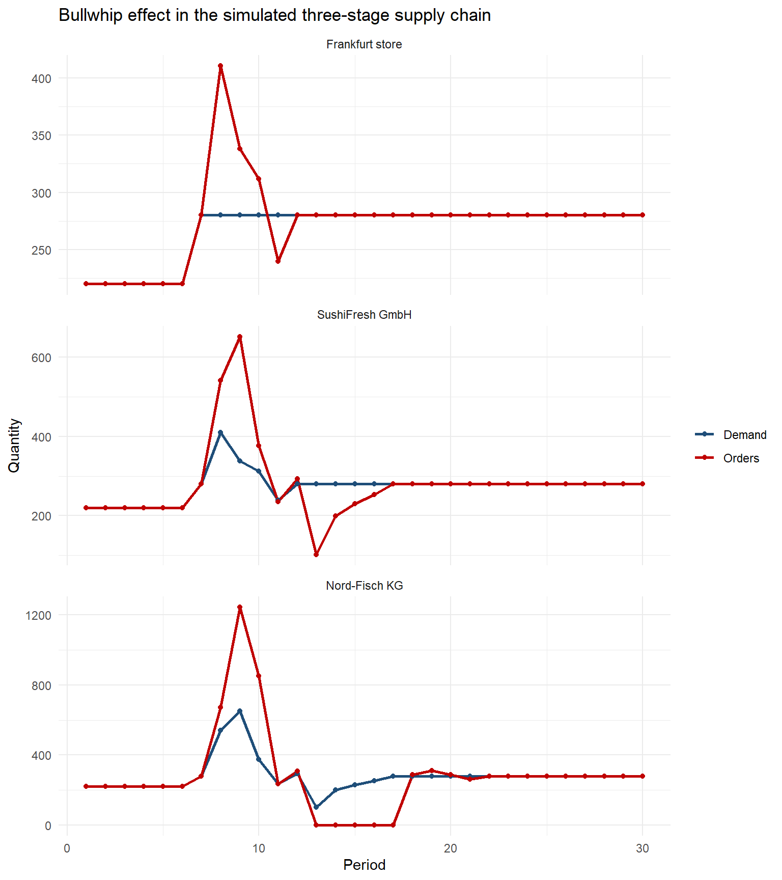
To make the effect visible graphically as well, we first bring the matrices into long format with pivot_longer() and then display a separate subplot for each stage. This is exactly what facet_wrap() from ggplot2 is made for: it automatically creates one panel per value of a grouping variable – here one subplot per stage of the chain:

sim_daten <- tibble(
  Periode    = rep(seq_len(n_perioden), times = n_stufen),
  Stufe      = factor(rep(stufen, each = n_perioden), levels = stufen),
  Demand     = as.vector(beobachtete_nachfrage),
  Orders     = as.vector(bestellung)
) |>
  pivot_longer(
    cols      = c(Demand, Orders),
    names_to  = "Series",
    values_to = "Menge"
  )

ggplot(sim_daten, aes(x = Periode, y = Menge, color = Series)) +
  geom_line(linewidth = 1) +
  geom_point(size = 1.5) +
  facet_wrap(~ Stufe, ncol = 1, scales = "free_y") +
  scale_color_manual(values = c(Demand = farbe_nachfrage, Orders = farbe_bestellung)) +
  labs(
    title = "Bullwhip effect in the simulated three-stage supply chain",
    x = "Period", y = "Quantity", color = NULL
  ) +
  theme_minimal()

The graph clearly shows how the initial demand step still arrives moderately at the Frankfurt store, but already strongly exaggerated at Nord-Fisch KG – the order quantity “overshoots” more strongly with each stage before settling at a new level again. Precisely this pattern – not the absolute level of the orders – is the characteristic “whip shape” that gives the bullwhip effect its name.

9.10 Lead time effects

The simulation already suggests that the replenishment lead time \(l\) is a central adjusting screw of the bullwhip effect. This can also be justified analytically: if the estimated demand rate \(\hat\mu\) changes by \(\Delta\hat\mu\) – for instance because a single high demand value slips into the rolling estimation window –, the order-up-to level changes according to the formula \(S=\hat\mu\cdot(l+1)+z_\alpha\hat\sigma\sqrt{l+1}\) by

\[ \Delta S = \Delta \hat\mu \cdot (l+1), \]

and this change is translated immediately and in full into a changed order quantity via the ordering rule \(q_t = S - p_t\). The longer the replenishment lead time, the larger the multiplier \((l+1)\) – and the more strongly the order quantity reacts to every forecast change, however small. The safety stock term also grows with \(\sqrt{l+1}\), albeit less than proportionally to the base demand term. We can make this relationship visible directly with diff() from the first R aside by calculating the order-up-to level for increasing replenishment lead times and determining the marginal increase per additional lead-time day:

# Demand parameters of the Frankfurt store (mu = 280, sigma = 55)
mu_beispiel    <- 280
sigma_beispiel <- 55

tibble(
  Lead_time = 0:4,
  Target_S = mu_beispiel * (0:4 + 1) +
    z_alpha * sigma_beispiel * sqrt(0:4 + 1)
) |>
  mutate(
    # marginal increase of the order-up-to level per additional lead-time day
    Marginal_increase = c(NA, diff(Target_S))
  ) |>
  kable(digits = 1, align = "r")

Lead_time	Target_S	Marginal_increase
0	370.5	NA
1	687.9	317.5
2	996.7	308.8
3	1300.9	304.2
4	1602.3	301.4

The table shows: with each additional day of replenishment lead time, the required order-up-to level rises – and with it the range within which order quantities can fluctuate. Shorter lead times therefore have a double effect: they not only reduce the required safety stock (we already know this from the pooling chapter) but also dampen the transmission of forecast fluctuations along the chain.

9.11 Causes of the bullwhip effect

The derivation so far already explains the bullwhip effect completely from the interplay of inventory policy, rolling forecasts and replenishment lead time. The seminal work by Lee et al. (1997) distinguishes four causes, which usually overlap in practice:

Demand signalling / forecast updating. Each stage wrongly interprets the order quantity of the downstream stage as an independent demand signal and updates its forecast on that basis – exactly the mechanism we reproduced in the simulation above. Since the order quantity itself is already a distorted, smoothed or delayed version of end-customer demand, the forecast error increases with each stage.

Order batching. For reasons of ordering costs, transport capacities (lot sizes, truckloads) or periodic ordering cycles, many companies do not order continuously but in bundled, larger lots. As a result, artificial demand peaks that do not actually exist appear to the upstream stage.

Price fluctuations and promotions. Temporary price reductions or special promotions lead customers – end consumers as well as business buyers – to engage in forward buying: they buy considerably more in the promotion period than they need in the short term, and correspondingly less in the following period. The observed demand therefore fluctuates more strongly than actual consumption would justify.

Rationing and shortage gaming. If – for instance because of a supply bottleneck – the supplier makes a proportional allocation (rationing), customers have an incentive to inflate their order quantities strategically in order to be allocated enough goods despite rationing. As soon as the situation eases, surplus orders are cancelled – what remains for the supplier is a seemingly highly volatile but in truth strategically distorted demand.

The lecture breaks these four root causes down into a more detailed overview of eight mechanisms, which is well suited as a checklist in practice:

Cause	Mechanism of action	Classification according to Lee et al.
Local forecasts	Orders are interpreted as actual demand	Demand signalling
Forecast updating	Small changes in demand lead to adjustments of target inventories	Demand signalling
Long lead times	Decisions must take effect far into the future (multiplier \(l+1\))	Demand signalling (amplifying)
Order batching	Infrequent large orders create artificial demand peaks	Order batching
Price promotions	Stockpiling purchases distort observed demand	Price fluctuations
Rationing	Actors strategically order more than their actual requirement	Shortage gaming
Lack of transparency	End-customer demand is not visible to all stages	cross-cutting
Local systems of objectives	Stages optimise individually instead of system-wide	cross-cutting

All four causes have in common that they are based on missing or delayed information about actual end-customer demand and that each stage optimises exclusively locally – in its own interest and with its own incomplete information – without considering the repercussions on the entire chain.

9.12 Empirical findings and consequences

The bullwhip effect is not a theoretical construct but has been documented empirically many times. In a sample of 4,689 listed US companies, around two thirds showed a positive amplification of procurement variability relative to sales variability (Bray and Mendelson 2012). The mean amplification amounted to 15.8% of demand variability, the median 6.7% – the distribution is therefore right-skewed: a few companies show a very strong effect. In absolute terms, the quarterly standard deviation of upstream orders was on average around US$20 million above that of observed demand. Complementary studies show that a stronger bullwhip effect is systematically associated with higher inventories and at the same time more shortages (Yao et al. 2020; Chen and Lee 2012) – so safety stocks alone do not compensate for the additional uncertainty. It is also noteworthy that metrics calculated at an aggregated level (e.g. monthly or category data) systematically underestimate the actual bullwhip effect at the level of individual items and weeks (Yao et al. 2020) – anyone wishing to measure the effect in their own company should therefore proceed as granularly as possible. Studies of real supplier networks – for instance in the Toyota production network – also confirm that the structure of a supply chain (number of stages, concentration of suppliers) significantly shapes the transmission and amplification of fluctuations (Kito et al. 2014).

As a management message, the lecture summarises: it is not only end-customer demand that generates volatility, but demand signal + local replenishment planning = order variance. The operational and economic consequences of the bullwhip effect are manifold:

Operational consequences	Economic consequences
Fluctuating production schedules	Higher capital tied up
Unstable capacity utilisation	Higher warehousing costs
Express shipments and special measures	Higher obsolescence risks
High inventories and yet shortages	Higher set-up and production costs
Lower delivery capability	Higher transport costs
Greater planning uncertainty	Losses in revenue and contribution margin

9.13 Countermeasures

Since the causes of the bullwhip effect lie above all in missing information and local optimisation, the most effective countermeasures start precisely there:

Lever	Measure	Effect
Information flow	Share point-of-sale (POS) data with upstream stages	reduces the forecast error at each stage
Inventory responsibility	Vendor Managed Inventory (VMI): the supplier manages its customer’s inventory itself	avoids duplicate, counteracting inventory adjustments
Joint planning	CPFR (Collaborative Planning, Forecasting and Replenishment): customer and supplier create a joint forecast	reduces local forecast distortions
Ordering policy	small, frequent instead of large, infrequent orders	reduces order batching effects
Lead time	shorten information and delivery lead times (e.g. through EDI, electronic data interchange)	reduces the protection period and thus the amplification factor \((l+1)\)
Pricing policy	stable prices instead of frequent promotions (every-day low pricing)	reduces artificial demand peaks caused by forward buying
Allocation	rationing based on historical sales volumes instead of current order quantities	reduces incentives for shortage gaming
Control logic	aim for the overall optimum instead of purely local targets	coordinates ordering and inventory decisions across the entire chain

The common denominator of these measures is coordination: the more information a stage receives about actual end-customer demand – instead of only about the (already distorted) orders of its direct neighbouring stage – the smaller the forecast error becomes, and the lower the amplification along the chain (Lee et al. 1997; Chopra and Meindl 2025). Precisely this insight is one of the most important drivers of the IT-based integration of supply chains, which today is standard via ERP systems, electronic data interchange and joint planning platforms.

9.14 Summary

This chapter has shown that a seemingly harmless, rational inventory policy – the order-up-to approach from the previous chapters – systematically leads to an amplification of demand fluctuations as soon as it is applied across several stages in succession: the bullwhip effect. We defined this effect formally, measured it with the variance ratio \(B=\operatorname{Var}(q_t)/\operatorname{Var}(d_t)\) and reproduced it in our own R simulation of a multi-echelon supply chain – the core of the classic Beer Game. The four classic causes (demand signalling, order batching, price fluctuations, rationing) explain why the effect occurs even when all participants behave rationally, while empirical studies document its considerable economic significance. Countermeasures such as information sharing, VMI and CPFR consistently address the underlying cause: a lack of transparency about actual demand.

On the R side, in this chapter you have learned to understand time series as simple vectors and to calculate period-to-period changes with diff(), to shift time series against each other with dplyr::lag(), to program a multi-echelon simulation as a nested loop, and to display the results of several groups clearly side by side with facet_wrap().

Review questions

1. Define the bullwhip effect and explain why a variance ratio \(B>1\) indicates it.
2. Why can the bullwhip effect occur even when each stage of a supply chain orders completely rationally according to an order-up-to rule?
3. Name and explain the four classic causes of the bullwhip effect according to Lee, Padmanabhan and Whang.
4. How does a longer replenishment lead time \(l\) affect the strength of the bullwhip effect, and why?
5. Describe the set-up and aim of the Beer Game. Which central insight of supply chain management does it make tangible?
6. Explain the difference between diff() and dplyr::lag() when working with time series in R.
7. What does the term Vendor Managed Inventory (VMI) mean, and to what extent does it reduce the bullwhip effect?
8. Calculate the lower bound of the variance ratio according to Chen et al. for \(L = 2\) and an estimation window of \(p = 3\) and \(p = 10\) periods respectively. What follows from this for the choice of forecasting method?
9. Why do participants in the Beer Game systematically order too much as soon as shortages have occurred? Explain the term supply line underweighting.
10. Outline in your own words how a multi-echelon simulation loop in R must be structured so that each stage uses the orders of the respective downstream stage as its own demand.

9.15 Outlook

With the bullwhip effect, this book comes full circle to a topic that has implicitly accompanied all the preceding chapters: dealing with uncertainty in supply chains. Location decisions, cost structures, pooling effects and the newsvendor model have shown how individual stages and individual decisions can be optimised under uncertain demand; the bullwhip effect makes clear that the sum of locally optimal decisions can destabilise a supply chain as a whole if information is not shared.

In business practice, this tension is not addressed with a single model but with a bundle of coordination mechanisms that have already been touched on in this chapter: the systematic sharing of sales data, joint demand planning (CPFR), the transfer of inventory responsibility to suppliers (VMI) and continuous IT-based integration of supply chain partners. These mechanisms do not replace the quantitative models developed in this book – rather, they are the organisational and technical infrastructure within which parameters such as \(\mu\), \(\sigma\) and \(l\) can be estimated reliably at all and the formulae derived here can be applied meaningfully. Anyone who masters these methods – from location choice and inventory planning to the analysis of multi-echelon chains – and can confidently use the R tools introduced in this book has a solid foundation for both penetrating supply chain problems quantitatively in practice and communicating and solving them in a team.

Bray, Robert L., and Haim Mendelson. 2012. “Information Transmission and the Bullwhip Effect: An Empirical Investigation.” Management Science 58 (5): 860–75. https://doi.org/10.1287/mnsc.1110.1467.

Cachon, Gérard, and Christian Terwiesch. 2024. Matching Supply with Demand: An Introduction to Operations Management. 5th ed. McGraw Hill.

Chen, Frank, Zvi Drezner, Jennifer K. Ryan, and David Simchi-Levi. 2000. “Quantifying the Bullwhip Effect in a Simple Supply Chain: The Impact of Forecasting, Lead Times, and Information.” Management Science 46 (3): 436–43.

Chen, Li, and Hau L. Lee. 2012. “Bullwhip Effect Measurement and Its Implications.” Operations Research 60 (4): 771–84.

Chopra, Sunil, and Peter Meindl. 2025. Supply Chain Management: Strategy, Planning, and Operation. 8th ed. Pearson.

Forrester, Jay W. 1961. Industrial Dynamics. MIT Press.

Kito, Tomomi, Alexandra Brintrup, Steve New, and Felix Reed-Tsochas. 2014. The Structure of the Toyota Supply Network: An Empirical Analysis. https://doi.org/10.2139/ssrn.2412512.

Lee, Hau L., V. Padmanabhan, and Seungjin Whang. 1997. “The Bullwhip Effect in Supply Chains.” Sloan Management Review 38 (3): 93–102.

Sterman, John D. 1989. “Modeling Managerial Behavior: Misperceptions of Feedback in a Dynamic Decision Making Experiment.” Management Science 35 (3): 321–39.

Yao, Yuliang, Yongrui Duan, and Jiazhen Huo. 2020. “On Empirically Estimating Bullwhip Effects: Measurement, Aggregation, and Impact.” Journal of Operations Management 67 (1): 5–30. https://doi.org/10.1002/joom.1090.