# Facility Location Planning II – Discrete Network Planning Models {#sec-standort-2}
```{r}
#| label: ch5-setup
#| echo: false
#| warning: false
#| message: false
# Load functions from scm_functions.R (incl. vogels_approximation(),
# .wlp_cost(), add_heuristic_wlp(), drop_heuristic_wlp())
source("../R/scm_functions.R")
library(tidyverse)
library(knitr)
library(kableExtra)
```
::: {.lernziele}
**Learning objectives**
After working through this chapter, you will be able to …
- distinguish discrete facility location and network planning problems from the continuous methods in Chapter [-@sec-standort-1],
- formulate the classical transportation problem as a linear optimisation model and solve it approximately with Vogel's approximation method,
- set up the warehouse location problem (WLP) as a mixed-integer optimisation model and interpret its decision variables, objective function and constraints,
- solve a WLP exactly with the R package `ompr` and interpret the result in economic terms,
- understand the basic ideas of constructive add and drop heuristics, apply them in R and assess their solution quality,
- test the sensitivity of a location decision to model assumptions (e.g. the scaling-up of demand),
- use lists, `purrr::map()` and matrices as R tools for structuring and analysing network planning data,
- position qualitative pre-selection methods (Chapter [-@sec-standort-1]) and quantitative cost optimisation as **complementary** building blocks of a location decision.
**Further reading**
- **Transportation, transhipment and network models:** [@guenther2012produktion, Chapter 4].
- **Discrete location models, algorithms and applications:** Chapters 1–4 in [@daskin2013network].
- **Theory and applications of facility location planning:** [@drezner2002facility] and [@kik2022standortplanung].
:::
## From continuous to discrete facility location planning
In the previous chapter you learnt how to use the centre-of-gravity approach and the Weiszfeld algorithm to determine an *arbitrary* point in the plane that minimises the weighted distances to a set of demand points. In the example of **SushiFresh GmbH** – a regional producer of fresh sushi boxes in the Rhine-Main area that supplies six supermarket stores every day – the optimal point calculated in this way lay between Raunheim and Frankfurt, shifted clearly towards Frankfurt, the store with the highest demand. This continuous view of location choice is analytically elegant but of limited help in business practice: SushiFresh cannot build a production facility at exactly the calculated coordinates but has to choose among the commercial plots, halls or existing properties that are actually available. Planning law, land prices, transport links and food hygiene requirements restrict the set of realistically usable locations to a **finite set of alternatives known in advance**. This is precisely the starting point of **discrete facility location planning**: instead of an optimisation problem over the entire plane $\mathbb{R}^2$, the focus is on a **selection decision** from a fixed list of potential locations.
In Chapter [-@sec-standort-1] the location question for SushiFresh was already addressed twice: first, a qualitative assessment of three candidate locations was carried out using the **AHP** (*Analytic Hierarchy Process*) – with the result that **Mainz-Hechtsheim** came out narrowly ahead of Raunheim, although the criteria weights were based on judgements that were not entirely consistent. Subsequently, the **centre-of-gravity/Weiszfeld approach** delivered a continuous optimal point in the middle of the sales area. This chapter poses the location question a third time – now on the basis of hard **cost figures**: fixed costs for operating a location and variable transport costs to the stores supplied. As we shall see, a purely cost-based, discrete analysis arrives at a different result from the qualitative pre-selection – and precisely this tension between the two methods is discussed explicitly at the end of the chapter.
::: {.definition}
**Definition: Discrete facility location planning**
In discrete facility location planning, the subset of a finite set of predefined potential locations is selected that minimises a given target value (usually the sum of fixed location costs and variable transport costs). In contrast to continuous facility location planning, the solution space is no longer continuous but **combinatorial**: every possible subset of locations represents a feasible solution.
:::
Discrete location decisions are always embedded in a larger **supply chain network**, which can be roughly divided into the stages of procurement, production, distribution and sales. At each of these stages, nodes (supplier plants, production facilities, warehouses, cross-docking points) can be opened, closed or connected with one another; in this context one also speaks of **network design**. The lecture emphasises that in practice usually only a **section** of the overall network is considered: specific locations are selected at one or two stages while the remaining stages are held fixed. Accordingly, this chapter concentrates on the question of which production and distribution locations SushiFresh should operate and which store should be supplied from which location. The models presented can, however, be transferred directly to other network stages.
We approach discrete facility location planning in two steps. First, we consider the **special case** in which the locations are already fixed and only the delivery quantities have to be optimally allocated to the stores – the classical **transportation problem**. We then extend the model to include the actual location decision: the **warehouse location problem (WLP)**, in which both the question “where?” and the question “how much to where?” have to be answered simultaneously.
## Case example: SushiFresh GmbH
::: {.fallstudie}
**Case study: Decision situation**
SushiFresh has to decide which candidate locations are to be developed for production and distribution and which store is to be supplied from which location. The company wants to make the decision in such a way that the annual total costs of fixed costs and transport are minimised. Compared with Chapter [-@sec-standort-1], the list of candidates has been extended by two further commercial sites: **Frankfurt-Höchst** and **Neu-Isenburg**, both located closer to the high-demand stores in the east of the sales area.
:::
The six stores (demand nodes $j$, referred to as C1–C6 in the lecture) with their mean daily demand $\mu_j$ and the demand standard deviation $\sigma_j$, which we will only encounter again in Chapter [-@sec-unsicherheit-pooling]:
```{r}
#| label: ch5-filialen-tabelle
filialen_fall <- tibble(
  ID    = paste0("C", 1:6),
  Filiale = c("Wiesbaden", "Mainz", "Frankfurt", "Ruesselsheim", "Darmstadt", "Offenbach"),
  lat   = c(50.0782, 50.0000, 50.1109, 49.9904, 49.8728, 50.0956),
  lon   = c(8.2398, 8.2711, 8.6821, 8.4116, 8.6512, 8.7761),
  mu    = c(120, 150, 280, 90, 110, 95),
  sigma = c(25, 30, 55, 20, 24, 22)
)

filialen_fall |>
  kbl(col.names = c("ID", "Store", "Latitude", "Longitude", "μ (boxes/day)", "σ")) |>
  kable_styling(bootstrap_options = c("striped", "condensed"), full_width = FALSE)
```
The five candidate locations (supply nodes $i$, S1–S5) with their fixed costs: the amounts of €180,000 to €260,000 mentioned in Chapter [-@sec-standort-1] are one-off investment and site development costs. For an annual model they are – in simplified form, without interest – spread linearly over a useful life of five years. This gives the annual fixed costs $f_i$:
```{r}
#| label: ch5-standorte-tabelle
standorte_fall <- tibble(
  ID          = paste0("S", 1:5),
  Standort    = c("Wiesbaden-Erbenheim", "Mainz-Hechtsheim", "Raunheim",
                  "Frankfurt-Hoechst", "Neu-Isenburg"),
  lat         = c(50.0632, 49.9698, 50.0000, 50.11146, 50.0543),
  lon         = c(8.2999, 8.2831, 8.4650, 8.54218, 8.7072),
  Investition = c(180000, 210000, 260000, 240000, 200000)
) |>
  mutate(Fixkosten = Investition / 5)   # linear allocation over 5 years

standorte_fall |>
  kbl(col.names = c("ID", "Location", "Latitude", "Longitude",
                    "Investment (€)", "Fixed costs f_i (€/year)"),
      format.args = list(big.mark = ",", decimal.mark = ".")) |>
  kable_styling(bootstrap_options = c("striped", "condensed"), full_width = FALSE)
```
For the transport costs it is assumed that each box costs €0.02 per kilometre of road (proportional vehicle, personnel and refrigeration costs). The road distances and this cost rate yield the **transport cost matrix** $c_{ij}$ in € per box. For the case example it is given – as in the lecture – and simplified for teaching purposes; it is therefore not identical in every entry with the actual distances in the Rhine-Main area. The (non-executed) code that follows shows how to calculate real road distances yourself.
```{r}
#| label: ch5-kostenmatrix
transportkostensatz <- 0.02   # EUR per box and kilometre

# Transport costs c_ij in EUR per box (rows: locations S1-S5, columns: stores C1-C6)
kosten_mat <- matrix(
  c(0.12348, 0.41478, 0.47474, 0.55152, 0.85996, 0.18220,
    0.09206, 0.51490, 0.59168, 0.88578, 0.73856, 0.78004,
    0.48168, 0.27202, 0.17036, 0.54650, 0.44772, 0.12592,
    0.61176, 0.66708, 0.89392, 0.33502, 0.68526, 0.74242,
    0.50226, 0.87512, 0.90576, 0.60740, 0.32042, 0.11400),
  nrow = 5, byrow = TRUE,
  dimnames = list(standorte_fall$ID, filialen_fall$ID)
)

# Implied road distances in km (costs / cost rate)
round(kosten_mat / transportkostensatz, 1)
```
```{r}
#| label: ch5-osrm
#| eval: false
# Not executed (requires internet access): this is how the road
# distances can be calculated yourself with the OSRM routing service.
library(osrm)
tab <- osrmTable(
  src = standorte_fall[, c("lon", "lat")],
  dst = filialen_fall[, c("lon", "lat")],
  measure = "distance"
)
dist_km <- tab$distances / 1000
```
::: {.callout-note}
## Note on reading the matrix
In real applications, a transport cost matrix is neither symmetric nor based on straight-line distance: roads, motorway junctions and Rhine bridges determine the actual distance, and travel times can vary greatly depending on the time of day. Such effects are the reason why discrete models in practice work with road distances or travel times rather than Euclidean distances – and why the continuous methods in Chapter [-@sec-standort-1] provide only an initial orientation.
:::
## The classical transportation problem
Let us first assume that SushiFresh – hypothetically, as a starting scenario *before* the actual location decision – already operates **all five** locations simultaneously and “only” has to decide which store is supplied from which location and with what quantity. The locations have limited daily production capacities which in total correspond exactly to the total demand of all six stores:
```{r}
#| label: ch5-angebot
angebot   <- c(S1 = 200, S2 = 150, S3 = 250, S4 = 120, S5 = 125)   # boxes/day
nachfrage <- setNames(filialen_fall$mu, filialen_fall$ID)          # boxes/day

c(Supply = sum(angebot), Demand = sum(nachfrage))
```
Five **sources** (supply of the locations) and six **sinks** (demand of the stores) – the classical **transportation problem**.
::: {.definition}
**Definition: Transportation problem**
In the (classical) transportation problem, $m$ sources $i \in I$ with supply quantities $s_i$ and $n$ sinks $j \in J$ with demand quantities $a_j$ are given. For each connection $(i,j)$, transport costs $c_{ij}$ are incurred per unit transported. The task is to find a cost-minimal allocation of the supply quantities to the demand quantities. The problem is called **balanced** if $\sum_i s_i = \sum_j a_j$ holds; otherwise it is **unbalanced**.
:::
Formally, the corresponding linear optimisation model with the transport quantities $x_{ij} \geq 0$ as decision variables reads:
$$
\begin{align}
\min \quad & \sum_{i \in I} \sum_{j \in J} c_{ij} \cdot x_{ij} \\
\text{s.t.} \quad & \sum_{j \in J} x_{ij} \leq s_i & \forall i \in I \quad &\rightarrow \text{supply constraint} \\
& \sum_{i \in I} x_{ij} = a_j & \forall j \in J \quad &\rightarrow \text{meet demand exactly} \\
& x_{ij} \geq 0 & \forall (i,j) &\quad \rightarrow \text{non-negativity}
\end{align}
$$
Since all constraints and the objective function are linear in $x_{ij}$, this is a pure **linear optimisation problem** (not an MILP) – the optimal solution always lies at a vertex of the solution polyhedron, and specialised, very efficient solution methods exist.
::: {.vertiefung}
**In depth (theory): Why transportation problems yield integer solutions “by themselves”**
The constraint matrix of the transportation problem has a special structure: each variable $x_{ij}$ appears in exactly two constraints – once in the supply row of $i$ and once in the demand row of $j$ – each time with the coefficient 1. Matrices with this structure are **totally unimodular**, i.e. every square submatrix has the determinant 0, +1 or −1. By Cramer's rule it follows that every vertex of the solution polyhedron is integer, provided the supply and demand quantities are integer. In practice this means: although the transportation problem is solved as an LP with continuous variables, one automatically obtains integer transport quantities – there is no need to round “half boxes” afterwards.
A second useful property concerns the number of positive transport quantities: a basic solution of a balanced transportation problem has at most $m + n - 1$ positive variables. With five locations and six stores, at most ten of the thirty possible connections are therefore used – most stores are supplied by exactly one location, and only a few are “split” between two locations. The opening procedures below generate precisely such basic solutions.
:::
Historically, so-called **tableau methods** were developed for transportation problems; they build on the simplex idea but exploit the special structure. Two classical opening procedures that construct an initial feasible solution are the **north-west corner method** and **Vogel's approximation method**.
The north-west corner method is extremely simple: one starts in the “north-west corner” of the tableau (row 1, column 1), supplies as much as possible there, deletes the row or column thereby exhausted and repeats the procedure for the remaining matrix. Its great advantage is its simplicity; its drawback: the costs $c_{ij}$ are **not taken into account at all** when choosing the cells. The method therefore always delivers a feasible, but often economically poor, starting solution.
**Vogel's approximation method (VAM)** improves on this by giving priority in each step to the row or column where a “wrong” decision would be most expensive. To do this, a **penalty cost difference** (*penalty*) is calculated for each row and each column: the difference between the two lowest costs in that row or column. A large difference means: if the cheapest cell is not chosen here, it becomes disproportionately expensive (opportunity cost of the second-best choice). The basic idea can be summarised as follows:
```r
# Core idea of Vogel's approximation method (simplified):
# Repeat as long as supply and demand remain open:
#   1. For each active row/column, calculate the penalty cost difference
#      = difference between the two lowest costs in that
#        row or column
#   2. Choose the row/column with the LARGEST penalty cost difference
#   3. In it, supply the cheapest cell with the maximum possible
#      quantity (= min(remaining supply, remaining demand))
#   4. Update remaining supply/demand; if a row/column is
#      exhausted, it is removed from further consideration
```
::: {.r-exkurs}
**R aside: Matrices as cost and transport tableaus**
So far you have mainly encountered tabular data as a `data.frame`/`tibble`, in which each column represents a named attribute vector with distinct content (e.g. place, longitude, demand). A cost or transport tableau, by contrast, is a **homogeneous, purely numerical table** in which what matters is not column names in the substantive sense but the *position* (row $i$, column $j$). The R data type **matrix** (`matrix()`) is the natural choice for this – as with `kosten_mat` above. Rows and columns can be named via `dimnames` and then addressed directly:
```{r}
#| label: ch5-matrix-zugriff
kosten_mat["S3", ] # all cost rates of Raunheim
kosten_mat[, "C3"] # costs of supplying Frankfurt from each location
apply(kosten_mat, 2, which.min) # per store: row index of the cheapest location
```
After solving, `rowSums()` and `colSums()` make it very easy to check whether a calculated allocation matrix is feasible: the row sums must equal the supply, the column sums the demand.
:::
The function `vogels_approximation()` from `R/scm_functions.R` implements the procedure outlined above in full, including automatic balancing via a dummy location or dummy store if supply and demand do not match:
```{r}
#| label: ch5-vogel-example
vam_ergebnis <- vogels_approximation(
  cost_mat = kosten_mat,
  supply   = angebot,
  demand   = nachfrage,
  verbose  = FALSE
)

vam_ergebnis$allocation
round(vam_ergebnis$total_cost, 2) # transport costs in EUR/day
# Feasibility check
rowSums(vam_ergebnis$allocation) == angebot
colSums(vam_ergebnis$allocation) == nachfrage
```
The allocation matrix shows an economically plausible picture: the stores are mainly supplied by the nearby locations, and only where a location has already exhausted its capacity is a store split between two locations. Total costs amount to €`r round(vam_ergebnis$total_cost, 2)` per day. Since VAM is an **opening heuristic**, this result need not be the optimal solution. How good it is can be checked by additionally solving the transportation problem exactly as an LP (with the package `ompr`, which is introduced in detail further below):
```{r}
#| label: ch5-transport-lp
#| message: false
library(ompr)
library(ompr.roi)
library(ROI.plugin.glpk)

m <- nrow(kosten_mat); n <- ncol(kosten_mat)

tp_modell <- MIPModel() |>
  add_variable(x[i, j], i = 1:m, j = 1:n, type = "continuous", lb = 0) |>
  set_objective(sum_expr(kosten_mat[i, j] * x[i, j], i = 1:m, j = 1:n), "min") |>
  add_constraint(sum_expr(x[i, j], j = 1:n) <= angebot[i], i = 1:m) |>
  add_constraint(sum_expr(x[i, j], i = 1:m) == nachfrage[j], j = 1:n)

tp_loesung <- solve_model(tp_modell, with_ROI(solver = "glpk"))
tp_opt     <- objective_value(tp_loesung)

c(VAM = round(vam_ergebnis$total_cost, 2), Optimum = round(tp_opt, 2),
  Deviation_percent = round((vam_ergebnis$total_cost / tp_opt - 1) * 100, 2))
```
`r if (abs(vam_ergebnis$total_cost - tp_opt) < 0.01) 'In this example, VAM actually finds the optimal solution straight away – this is not guaranteed, but it happens frequently with small instances because the penalty cost logic deliberately avoids the expensive wrong decisions.' else paste0('In this example, the VAM solution lies ', round((vam_ergebnis$total_cost / tp_opt - 1) * 100, 1), '% above the optimum – a typical value for opening procedures.')` The transportation problem, however, assumes that the set of supplying locations is already fixed. It is precisely this assumption that is relaxed in the next section.
## The warehouse location problem
In practice, it usually has to be clarified not only *how* stores are supplied but also *from which* locations deliveries should be made at all. For SushiFresh this is the actual strategic question: is it worth operating several locations simultaneously, or is **consolidation** onto one or two locations cheaper? Every location opening entails a fixed annual cost burden, regardless of how much is later actually delivered via this location. This decision problem is called the **warehouse location problem (WLP)** or also the **uncapacitated facility location problem** if – as here – no capacity limits per location are assumed.
::: {.definition}
**Definition: Warehouse location problem**
Let there be a set of potential locations $i \in I$ with annual opening costs $f_i$ and a set of customer locations $j \in J$ with demand quantities $a_j$. For each possible transport connection $(i,j) \in E \subseteq I \times J$, transport costs $c_{ij}$ are incurred per unit supplied. The task is to find the subset of locations to be opened and the corresponding assignment of customers to locations that minimises the sum of opening and transport costs.
:::
In contrast to the transportation problem, the WLP now contains **two types of decision variables**: a binary location decision $y_i \in \{0,1\}$ (location $i$ is opened or not) and, as before, the continuous transport quantities $x_{ij} \geq 0$. The complete model reads:
$$
\min \rightarrow \sum_{i \in I} y_i \cdot f_i + \sum_{(i,j) \in E} x_{ij} \cdot c_{ij}
$$
subject to the constraints
$$
\begin{align}
\sum_{(i,j) \in E} x_{ij} &= a_j & \forall j \in J &\quad\rightarrow \text{satisfy demand completely} \\
x_{ij} &\leq y_i \cdot a_j & \forall (i,j) \in E &\quad\rightarrow \text{only transports from opened locations} \\
x_{ij} &\geq 0 & \forall (i,j) \in E &\quad\rightarrow \text{transport quantities non-negative} \\
y_i &\in \{0,1\} & \forall i \in I &\quad\rightarrow \text{location is opened or not}
\end{align}
$$
The second constraint is the decisive difference from the pure transportation problem: as long as $y_i = 0$ (location $i$ not opened), it forces *all* associated transport quantities $x_{ij}$ to zero – a closed location cannot supply any store. Only when $y_i = 1$ is set is $x_{ij}$ permitted up to at most the full demand $a_j$. Because both continuous and binary variables appear in the same model, this is a **mixed-integer linear optimisation model** (*mixed-integer linear program*, MILP) – a considerably more difficult problem class than the pure LP of the transportation problem.
::: {.vertiefung}
**In depth (theory): Structure of the optimal solution and “strong” formulations**
Because the WLP has no capacity limits, its optimal solution has a simple structure: as soon as it is fixed which locations are open, each store is supplied **entirely from the cheapest open location**. Splitting a store between several locations can never be better, since every box should be transported on the cheapest available connection. The real difficulty of the problem therefore lies solely in the combinatorial selection of the set of locations – with $|I|$ candidates there are $2^{|I|}-1$ non-empty subsets. The add and drop heuristics and the helper function `.wlp_cost()` exploit precisely this observation.
For exact solution with an MILP solver, the formulation of the linking constraint is important. Instead of the **disaggregated** form $x_{ij} \leq y_i \cdot a_j$ used here (one constraint per connection), one could also write an **aggregated** form $\sum_j x_{ij} \leq y_i \cdot \sum_j a_j$ (one constraint per location). Both formulations have the same integer solutions. Solvers, however, work with the **LP relaxation**, in which $y_i$ may take values between 0 and 1. In the aggregated form, a very small $y_i$ then suffices to open a location “a little” and supply all stores through it – the relaxation provides a weak lower bound, and the branch-and-bound procedure has to search many branches. The disaggregated form, by contrast, requires $y_i \geq x_{ij}/a_j$ for each individual connection and is therefore much closer to the integer solution; this is referred to as a **strong formulation**. For the uncapacitated WLP, the LP relaxation of the disaggregated form is often already integer [@daskin2013network].
:::
Unlike the transportation problem in the previous section, we calculate the WLP on an **annual basis**: the fixed costs $f_i$ are annual values, and demand must also be scaled up from the daily to the annual level. The numerical example in the lecture uses the simplified factor 1,000 for this ($a_j = 1{,}000 \cdot \mu_j$). We adopt this assumption for now and check at the end of the chapter how sensitively the result reacts to a more realistic scaling-up with 365 sales days. Before we compile the data, it is worth looking at another central R concept: the **list**.
::: {.r-exkurs}
**R aside: Lists as a flexible data structure**
A vector in R can only hold elements of **one** data type, and a `data.frame`/`tibble` requires all columns to have the same length. Often, however, one wants to manage objects of different structure, length or type together – for instance the name of a location (text), its coordinates (a vector of length 2), its fixed costs (a number) and a status (logical). This is exactly what the **list** (`list()`) is intended for: a container whose elements may be any – including heterogeneous – R objects.
A named element is accessed either with the dollar sign `$name` or with double square brackets `[["name"]]` or `[[position]]`. The difference from single square brackets `[ ]` is important: `liste[1]` returns a *sub-list* with one element, `liste[[1]]` returns the *content* of that element itself.
```{r}
#| label: ch5-liste-basics
# A single piece of location information as a list
standort_info <- list(
  name        = "Wiesbaden-Erbenheim",
  koordinaten = c(lon = 8.2999, lat = 50.0632),  # vector as element
  fixkosten   = 36000,
  aktiv       = TRUE
)

standort_info$name                     # access via $
standort_info[["fixkosten"]] # access via [[ ]] with name
standort_info[["koordinaten"]]["lat"] # nested access
```
Lists are not only useful for *input* – the **return values** of many R functions are also lists as soon as more than one result is to be returned. We already made use of this in the previous section: `vogels_approximation()` returns a list with the fields `allocation` (matrix), `total_cost` (number) and `balanced` (logical). Likewise, `add_heuristic_wlp()` and `drop_heuristic_wlp()`, which we use further below, return their result as a list with the fields `open_warehouses`, `fixed_cost`, `transport_cost`, `total_cost` and `assignment`.
:::
For the actual calculation we need the fixed costs and the annual demand as **named vectors**, as well as the cost matrix `kosten_mat`:
```{r}
#| label: ch5-wlp-daten
fixkosten_vec  <- setNames(standorte_fall$Fixkosten, standorte_fall$ID)   # EUR/year
nachfrage_jahr <- setNames(filialen_fall$mu * 1000, filialen_fall$ID)     # boxes/year (factor 1,000)

fixkosten_vec
nachfrage_jahr
```
Five locations mean $2^5 - 1 = 31$ possible non-empty location configurations – small enough to evaluate them all in the next R aside.
::: {.r-exkurs}
**R aside: `purrr::map()` – applying a function to every element**
Often one wants to apply the same calculation to every element of a list or vector – for example: “calculate the total costs for every possible combination of locations”. Instead of writing a `for` loop for this (Chapter [-@sec-standort-1]), the `tidyverse` package `purrr` offers the `map()` family of functions. `map(x, f)` applies the function `f` to every element of `x` and returns a list; `map_dbl(x, f)` does the same but requires `f` to return a single number (`double`) per element, and then automatically simplifies the result to a numeric vector. It is the direct relative of `sapply()` from Chapter [-@sec-standort-1], with the advantage that the return type is clearly fixed and errors therefore become apparent earlier.
We first generate all non-empty subsets of the five locations with the base R function `combn()` and then evaluate them with `map_dbl()` and the helper function `.wlp_cost()` from `scm_functions.R`, which, for a given set of open locations, calculates the optimal store assignment (each store to the cheapest open location) and the resulting total costs:
```{r}
#| label: ch5-purrr-map
n_I <- length(fixkosten_vec)

# All non-empty subsets of {1, ..., 5}: combn(5, k) returns all
# combinations of size k, unlist(..., recursive = FALSE) merges them into
# a single list
alle_teilmengen <- unlist(
  lapply(1:n_I, function(k) combn(n_I, k, simplify = FALSE)),
  recursive = FALSE
)
length(alle_teilmengen)  # 2^5 - 1 = 31
# Calculate the total costs for each subset
kosten_je_teilmenge <- map_dbl(alle_teilmengen, function(S) {
  .wlp_cost(S, fixkosten_vec, kosten_mat, nachfrage_jahr)$total
})

beste_teilmenge <- alle_teilmengen[[which.min(kosten_je_teilmenge)]]
standorte_fall$Standort[beste_teilmenge]
round(min(kosten_je_teilmenge))
```
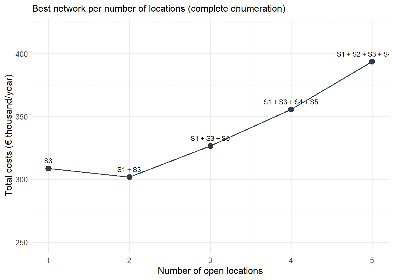
Complete enumeration shows that it is cheapest to operate **two** locations – **Wiesbaden-Erbenheim and Raunheim** – with total costs of around €`r format(round(min(kosten_je_teilmenge)), big.mark = ",", decimal.mark = ".")`/year. The ten best configurations at a glance:
```{r}
#| label: ch5-brute-force-tabelle
brute_force_df <- map_dfr(alle_teilmengen, function(S) {
  res <- .wlp_cost(S, fixkosten_vec, kosten_mat, nachfrage_jahr)
  tibble(
    Standorte       = paste(standorte_fall$ID[S], collapse = " + "),
    Anzahl          = length(S),
    Fixkosten       = res$fixed,
    Transportkosten = round(res$transport),
    Gesamtkosten    = round(res$total)
  )
}) |>
  arrange(Gesamtkosten)

brute_force_df |>
  head(10) |>
  kbl(col.names = c("Open locations", "Number", "Fixed costs (€)",
                    "Transport costs (€)", "Total costs (€/year)"),
      format.args = list(big.mark = ",", decimal.mark = ".")) |>
  kable_styling(bootstrap_options = c("striped", "condensed"), full_width = FALSE) |>
  row_spec(1, bold = TRUE, background = "#E8F4F1")
```
The ranking is revealing. First, the best solutions lie very close together: the combination Mainz-Hechtsheim + Raunheim and the **single location Raunheim** are only a few thousand euros per year more expensive than the optimum. Second, Raunheim appears in all the leading solutions – the location with the highest investment costs is the backbone of every good network because, according to the cost matrix, it reaches the high-demand Frankfurt store and most of the other stores most cheaply. Third, a second location in the west (Wiesbaden-Erbenheim) is only just worthwhile: it saves transport costs to the Wiesbaden store which only just exceed the additional fixed costs.
This brute-force search only works because $|I|=5$ is very small. With $|I|=20$ locations there would already be over a million subsets, with $|I|=50$ more than $10^{15}$ – a complete search is then hopeless even on powerful computers. Realistic instances therefore require either **efficient exact methods** or **heuristics**.
:::
## Exact solution with ompr
The WLP can be solved exactly as an MILP with specialised solvers without evaluating all subsets individually. In R, the package **`ompr`** (*Optimization Modeling Package for R*) handles the algebraic formulation of the model; the actual numerical solution is delegated via `ompr.roi` to a solver – here `glpk`, the free *GNU Linear Programming Kit*. The appeal of `ompr` lies in the fact that the objective function and constraints can be translated almost literally from the mathematical formulation into R code.
::: {.r-exkurs}
**R aside: Algebraic optimisation modelling with `ompr`**
So far we have solved optimisation problems (centre of gravity, Weiszfeld, Vogel's method) using **tailor-made algorithms**. `ompr` takes a more generic approach: the model is described **declaratively** (variables, objective function, constraints) and the search for a solution is left to a universal solver. The workflow is divided into six steps:
1. `MIPModel()` – create an empty model object,
2. `add_variable()` – define decision variables with type (`binary`, `continuous`, `integer`) and index set,
3. `set_objective()` – formulate the objective function (`sum_expr()` forms sums over index sets, analogous to $\sum$ in mathematical notation),
4. `add_constraint()` – formulate constraints, likewise indexed,
5. `solve_model()` – pass the model to a specific solver,
6. `get_solution()` – extract the optimal values of the decision variables from the result object.
In the following code, `y[i]` corresponds to the binary location variable $y_i$ and `x[i,j]` to the transport quantity variable $x_{ij}$. `sum_expr(f[i] * y[i], i = 1:n_I)` forms exactly the expression $\sum_{i\in I} f_i \cdot y_i$; the two `add_constraint()` calls implement the demand and linking constraints of the WLP model.
```{r}
#| label: ch5-ompr-model
n_J  <- length(nachfrage_jahr)
f    <- fixkosten_vec     # opening costs f_i (EUR/year)
a    <- nachfrage_jahr    # demand a_j (boxes/year)
c_ij <- kosten_mat        # transport costs (EUR/box)

modell <- MIPModel() |>
  # Decision variable y_i: open location i (1) or not (0)
  add_variable(y[i], i = 1:n_I, type = "binary") |>
  # Decision variable x_ij: transport quantity from location i to store j
  add_variable(x[i, j], i = 1:n_I, j = 1:n_J, type = "continuous", lb = 0) |>
  # Objective function: minimise opening costs + transport costs
  set_objective(
    sum_expr(f[i] * y[i], i = 1:n_I) +
      sum_expr(c_ij[i, j] * x[i, j], i = 1:n_I, j = 1:n_J),
    sense = "min") |>
  # C1: satisfy the demand of each store j completely
  add_constraint(sum_expr(x[i, j], i = 1:n_I) == a[j], j = 1:n_J) |>
  # C2: transport only from opened locations (x_ij <= y_i * a_j)
  add_constraint(x[i, j] <= y[i] * a[j], i = 1:n_I, j = 1:n_J)

ergebnis_milp <- solve_model(modell, with_ROI(solver = "glpk", verbose = FALSE))
```
:::
After solving, we use `get_solution()` to extract the optimal values of the variables $y_i$ and $x_{ij}$, and `objective_value()` to obtain the optimal objective function value $Z^*$:
```{r}
#| label: ch5-ompr-solution
y_sol <- get_solution(ergebnis_milp, y[i])
x_sol <- get_solution(ergebnis_milp, x[i, j])

offene_idx       <- y_sol$i[y_sol$value > 0.5]
offene_standorte <- standorte_fall$Standort[offene_idx]
offene_standorte
round(objective_value(ergebnis_milp))
```
```{r}
#| label: ch5-ompr-zuordnung
x_sol |>
  filter(value > 0.001) |>
  mutate(Standort = standorte_fall$Standort[i],
         Filiale  = filialen_fall$Filiale[j],
         Menge    = value,
         Transportkosten = round(c_ij[cbind(i, j)] * value)) |>
  select(Standort, Filiale, Menge, Transportkosten) |>
  kbl(col.names = c("Location", "Store", "Quantity x_ij (boxes/year)", "Transport costs (€/year)"),
      format.args = list(big.mark = ",", decimal.mark = ".")) |>
  kable_styling(bootstrap_options = c("striped", "condensed"), full_width = FALSE)
```
The solver confirms the result of the complete enumeration: **Wiesbaden-Erbenheim** and **Raunheim** are opened. Wiesbaden-Erbenheim supplies only the Wiesbaden store, while all other five stores are supplied from Raunheim – each store entirely from exactly one location, as theory predicts for the uncapacitated WLP. The decisive difference from enumeration is the **method of calculation**: `ompr`/`glpk` did not have to evaluate all 31 subsets individually but internally uses branch-and-bound and cutting-plane methods, with which even WLP instances with hundreds of locations and customers can be solved exactly in reasonable time.
## Heuristic solution methods: add and drop heuristics
Despite the power of modern MILP solvers, the WLP remains an **NP-hard** problem: in the worst case, the computing time required for an exact solution grows exponentially with the number of locations and customers. For very large practical instances – a Germany-wide store network with hundreds of candidate locations and thousands of stores, possibly with further constraints (capacities, multi-stage networks) – even a good solver can run into time or memory limits. In such cases, **constructive heuristics** are often the practicable route to a usable, though not necessarily optimal, solution.
The basic idea of both heuristics presented below is **greedy**: starting from a feasible initial configuration, in each step exactly the change that reduces total costs the most is made; the procedure stops as soon as no further improvement is possible. Stores are always assigned to the *cheapest open* location ($\sigma(j) = \arg\min_{i \in S} c_{ij}$), so that the total costs of a set of locations $S$ can be calculated unambiguously as
$$Z(S) = \underbrace{\sum_{i \in S} f_i}_{\text{opening}} + \underbrace{\sum_{j \in J} \min_{i \in S} c_{ij} \cdot a_j}_{\text{transport}}.$$
The **add heuristic** starts with the empty set $S = \emptyset$ and in each step adds the location $i^*$ whose opening reduces total costs the most: $\Delta_i = Z(S) - Z(S \cup \{i\})$, $i^* = \arg\max_{i \notin S} \Delta_i$. If $\Delta_{i^*} > 0$, $i^*$ is opened; otherwise the procedure terminates. In economic terms, adding a location is worthwhile precisely when the **transport cost savings** it achieves are greater than its **opening costs**. Transport costs fall from step to step, while fixed costs rise.
The **drop heuristic** takes the opposite route: it starts with *all* locations open ($S = I$) and in each step closes the location whose closure reduces total costs the most ($\Delta_i = Z(S) - Z(S \setminus \{i\})$), until here too no further improvement is possible. A location is closed if its fixed costs are higher than the transport costs incurred because its stores have to be reassigned to the next-best location.
| Feature | Add heuristic | Drop heuristic |
|:---|:---|:---|
| Start | $S = \emptyset$ (costs $\infty$) | $S = I$ (all fixed costs incurred) |
| Direction | constructive (building up) | destructive (reducing) |
| Effort per step | $\mathcal{O}(\lvert I \rvert \cdot \lvert J \rvert)$ | $\mathcal{O}(\lvert I \rvert \cdot \lvert J \rvert)$ |
| Tendency | rather few locations | rather more locations |
Both variants are implemented in `R/scm_functions.R` as `add_heuristic_wlp()` and `drop_heuristic_wlp()` respectively (including the internal cost calculation via `.wlp_cost()`). With `verbose = TRUE` they log each step:
```{r}
#| label: ch5-add-heuristik
names(fixkosten_vec) <- standorte_fall$Standort   # names for a readable log

add_ergebnis <- add_heuristic_wlp(
  fixed_costs        = fixkosten_vec,
  transport_cost_mat = kosten_mat,
  demand             = nachfrage_jahr,
  verbose            = TRUE
)
round(add_ergebnis$total_cost)
```
In the first step, the add heuristic opens **Raunheim** – the location that, on its own, incurs the lowest total costs of all single locations. In the second step, Wiesbaden-Erbenheim is added because the transport cost savings for the Wiesbaden store exceed the additional fixed costs. After that, no further location can reduce costs.
```{r}
#| label: ch5-drop-heuristik
drop_ergebnis <- drop_heuristic_wlp(
  fixed_costs        = fixkosten_vec,
  transport_cost_mat = kosten_mat,
  demand             = nachfrage_jahr,
  verbose            = TRUE
)
round(drop_ergebnis$total_cost)
```
The drop heuristic starts with all five locations open and successively closes Mainz-Hechtsheim, Frankfurt-Höchst and Neu-Isenburg – in each case the location whose fixed costs generate the least “transport benefit”. What remains are Wiesbaden-Erbenheim and Raunheim: **here the add and drop heuristics independently converge on the same, demonstrably optimal solution.** This is by no means a matter of course – with other cost structures, the two procedures can end in different, suboptimal solutions – but here it shows how clearly the cost structure of the case example points to this configuration.
```{r}
#| label: ch5-vergleich-tabelle
vergleich <- tibble(
  Verfahren = c("Optimum (MILP)", "Add heuristic", "Drop heuristic"),
  `Offene Standorte` = c(paste(offene_standorte, collapse = ", "),
                         paste(add_ergebnis$open_names, collapse = ", "),
                         paste(drop_ergebnis$open_names, collapse = ", ")),
  Fixkosten = c(sum(f[offene_idx]), add_ergebnis$fixed_cost, drop_ergebnis$fixed_cost),
  Gesamtkosten = round(c(objective_value(ergebnis_milp),
                         add_ergebnis$total_cost, drop_ergebnis$total_cost))
) |>
  mutate(Transportkosten = Gesamtkosten - Fixkosten,
         `Gap zum Optimum (%)` = round((Gesamtkosten / Gesamtkosten[1] - 1) * 100, 2))

vergleich |>
  kbl(col.names = c("Method", "Open locations", "Fixed costs", "Total costs",
                    "Transport costs", "Gap to optimum (%)"),
      format.args = list(big.mark = ",", decimal.mark = ".")) |>
  kable_styling(bootstrap_options = c("striped", "condensed"), full_width = FALSE)
```
```{r}
#| label: ch5-heuristik-verlauf
#| fig-cap: "Total costs as a function of the number of open locations: best network for each number of locations and the paths of the add and drop heuristics"
bestes_je_anzahl <- brute_force_df |>
  group_by(Anzahl) |>
  slice_min(Gesamtkosten, n = 1) |>
  ungroup()

ggplot(bestes_je_anzahl, aes(Anzahl, Gesamtkosten / 1000)) +
  geom_line(colour = "#2F3E46") +
  geom_point(size = 3, colour = "#2F3E46") +
  geom_text(aes(label = Standorte), vjust = -1, size = 3) +
  labs(x = "Number of open locations", y = "Total costs (€ thousand/year)",
       subtitle = "Best network per number of locations (complete enumeration)") +
  scale_y_continuous(limits = c(250, 420)) +
  theme_minimal(base_size = 12)
```
The figure shows the typical **U-shape** of total costs plotted against the number of locations – the same trade-off logic that was introduced in Chapter [-@sec-logistikkosten] as the “decision on the number of warehouses”: with each additional location, transport costs fall while fixed costs rise. The minimum lies at two locations, but the curve is very flat in the vicinity of the minimum.
For practice this means: the add and drop heuristics should – where possible – be run in parallel and compared with the result of an exact method (or at least a known lower bound) before a location decision with long-term binding effect is taken. Especially for distribution locations, which can only be revised at great expense, a reliable quality measure (the *gap* to the optimum) is indispensable [@chopra2025supply].
## How robust is the solution? A sensitivity analysis
The flat cost curve suggests that the optimal solution could react sensitively to assumptions. The most important assumption of the numerical example is the scaling-up of daily to annual demand by the factor 1,000. If SushiFresh sells on 365 days a year, the actual annual quantity – and hence the weight of transport costs relative to fixed costs – would be considerably smaller. With `map_dfr()` the optimum can be determined for different scaling factors:
```{r}
#| label: ch5-sensitivitaet
bestes_netz <- function(faktor) {
  a_tmp  <- filialen_fall$mu * faktor
  kosten <- map_dbl(alle_teilmengen, ~ .wlp_cost(.x, fixkosten_vec, kosten_mat, a_tmp)$total)
  S      <- alle_teilmengen[[which.min(kosten)]]
  tibble(Days_per_year = faktor,
         Optimal_network = paste(standorte_fall$Standort[S], collapse = " + "),
         Total_costs = round(min(kosten)))
}

map_dfr(c(250, 300, 365, 500, 750, 1000), bestes_netz) |>
  kbl(format.args = list(big.mark = ",", decimal.mark = ".")) |>
  kable_styling(bootstrap_options = c("striped", "condensed"), full_width = FALSE)
```
The result is instructive: with a realistic scaling-up based on 365 sales days, it is no longer the two-location solution but the **single location Raunheim** that is optimal. The lower the transport volume, the less worthwhile the fixed cost burden of a second location; only at considerably higher annual quantities does the additional proximity to the Wiesbaden store pay off. The sensitivity analysis thus shows that the question “one or two locations?” is finely balanced in the case example – while the role of **Raunheim as the central location** remains stable in all scenarios.
## Qualitative vs. quantitative location assessment
At this point it is worth looking back at Chapter [-@sec-standort-1]: there, the **AHP analysis** narrowly favoured **Mainz-Hechtsheim** among the three original candidates – mainly because of the very good rating for the availability of skilled labour there. The **quantitative cost optimisation** carried out in this chapter comes to a clearly different conclusion: Mainz-Hechtsheim does not appear in any of the best solutions; the cost-optimal choice is Raunheim (alone or together with Wiesbaden-Erbenheim).
```{r}
#| label: ch5-ahp-vs-milp
map_dfr(1:3, function(i) {
  res <- .wlp_cost(i, fixkosten_vec, kosten_mat, nachfrage_jahr)
  tibble(Location = standorte_fall$Standort[i], Fixed_costs = res$fixed,
         Transport_costs = round(res$transport), Total_costs = round(res$total))
}) |>
  kbl(caption = "The three original candidates as single locations (factor 1,000)",
      format.args = list(big.mark = ",", decimal.mark = ".")) |>
  kable_styling(bootstrap_options = c("striped", "condensed"), full_width = FALSE)
```
The reason for the discrepancy lies in the transport costs: Mainz-Hechtsheim lies on the western edge of the sales area, whereas the bulk of demand (above all Frankfurt) arises further east. The transport costs of a single location at Mainz-Hechtsheim are therefore far higher than those of Raunheim – a disadvantage that neither the lower fixed costs nor the good availability of skilled labour can offset, as long as the latter is not valued in euros.
This observation is not a contradiction but illustrates the **different function** of the two methods in the decision-making process: the AHP is suitable for an initial **pre-selection** based on criteria that are difficult to quantify and partly soft, and for incorporating different stakeholder perspectives. It does not, however, replace a robust **cost optimisation** as soon as hard figures are available. Conversely, a pure cost optimisation falls short if aspects that are difficult to monetise are ignored: if hardly any suitable skilled workers could actually be found in Raunheim, this would be reflected in higher personnel costs, quality problems or start-up difficulties of which the WLP knows nothing. In practice, the two methods complement each other: qualitative methods to reduce the search space and to check knock-out criteria, quantitative optimisation models for the final, cost-based decision between the remaining candidates.
::: {.fallstudie}
**Case study: Interim result for SushiFresh**
The WLP recommends a central location in **Raunheim**, possibly supplemented by a second location in Wiesbaden-Erbenheim. Since the two-location solution in the numerical example is only around €`r format(round(brute_force_df$Gesamtkosten[brute_force_df$Standorte == "S3"] - min(brute_force_df$Gesamtkosten)), big.mark = ",", decimal.mark = ".")`/year cheaper than the single location Raunheim, and is even more expensive with realistic scaling-up, there is much to be said for **consolidating production in a central kitchen in Raunheim**. However, the WLP ignores one important effect: the inventories that have to be held at each location as a safeguard against demand fluctuations. Precisely this question – how much safety stock does centralised supply save compared with decentralised supply? – is examined in Chapter [-@sec-unsicherheit-pooling]. It provides an additional, weighty argument in favour of consolidation.
:::
## Summary
This chapter has made the transition from continuous to **discrete facility location planning**: instead of an arbitrary point in the plane, a subset is sought from a finite list of predefined candidate locations. As a methodological starting point, we became acquainted with the **classical transportation problem**, in which the supplying locations are already fixed and only the transport flows have to be determined at minimum cost; its constraint matrix is totally unimodular, so that the LP solution is automatically integer. **Vogel's approximation method** delivers a good starting solution in a few steps by giving priority to supplying the row or column with the largest penalty cost difference.
The **warehouse location problem** extends this model to include the actual location decision: a binary variable $y_i$ per location decides on opening or not opening, linked to the transport quantities $x_{ij}$ via the constraint $x_{ij} \leq y_i \cdot a_j$. Because both binary and continuous variables occur, this is an MILP that can be solved exactly with `ompr` in a few lines of code closely modelled on the mathematical formulation. The SushiFresh example showed that the centrally located Raunheim site forms the backbone of every good network despite having the highest investment costs; whether a second location in Wiesbaden-Erbenheim is added depends – as the sensitivity analysis showed – on the scaling-up of demand. The qualitative AHP recommendation (Mainz-Hechtsheim) was not confirmed by the cost optimisation, which underlines the need for both methods in the decision-making process. Since the WLP is NP-hard, constructive **add** and **drop heuristics** are a practicable way out for large instances – in the case example both found the global optimum, although this is not a generally valid property of these methods.
On the R side, this chapter has introduced you to four new building blocks: **lists** as a flexible container for heterogeneous data and function results; **`purrr::map()`/`map_dbl()`/`map_dfr()`** for compactly applying a function to every element of a list; **matrices** as the natural representation of position-based tableaus, with `rowSums()`/`colSums()` for consistency checks; and **algebraic optimisation modelling** with `ompr`.
::: {.kontrollfragen}
**Review questions**
1. How does discrete facility location planning differ from continuous facility location planning, and why is the discrete variant more realistic for most practical location decisions?
2. Formulate the objective function and constraints of the classical transportation problem. What does it mean if a transportation problem is “unbalanced”, and how does `vogels_approximation()` deal with this?
3. Explain the basic idea of Vogel's approximation method. Why does it usually deliver better starting solutions than the north-west corner method?
4. Why does the LP solution of a transportation problem with integer supply and demand quantities automatically yield integer transport quantities?
5. Which additional decision variable does the warehouse location problem contain compared with the transportation problem, and what role does the constraint $x_{ij} \leq y_i \cdot a_j$ play? Why is it preferable to the aggregated form $\sum_j x_{ij} \leq y_i \sum_j a_j$?
6. Describe the add and drop heuristics in your own words. Under what condition is it worthwhile in the add heuristic to open a further location?
7. What is meant by the “gap to the optimum”, and why is it an important indicator for heuristic location decisions?
8. Explain the difference between a list (`list()`) and a `data.frame`/`tibble`. Give an example from this chapter in which an R function sensibly returns its result as a list.
9. Why, in the SushiFresh example, is one location optimal with 365 sales days, whereas two locations are optimal with 1,000 “days”? Argue on the basis of the structure of the objective function.
10. The AHP analysis (Chapter [-@sec-standort-1]) favours Mainz-Hechtsheim, the WLP analysis Raunheim. Explain the discrepancy and discuss how the two methods can be sensibly combined in practice.
:::