Supply Chain Management

Winter semester 2026/27

Matthias Kalverkamp & Thomas Kirschstein

Introduction & Course Organisation

Course organisation

Lecturers: Prof. Dr. Matthias Kalverkamp & Prof. Dr. Thomas Kirschstein
Documents + materials: https://github.com/tkirschstein/SCM
Case studies: 6 case studies in group work 3-6 persons
Exam: reflection report

Literature

Baumast, Annett, and Jens Pape, eds. 2013. Betriebliches Nachhaltigkeitsmanagement. UTB / Verlag Eugen Ulmer.

Bray, Robert L., and Haim Mendelson. 2012. “Information Transmission and the Bullwhip Effect: An Empirical Investigation.” Management Science 58 (5): 860–75. https://doi.org/10.1287/mnsc.1110.1467.

Buscher, Udo, Anke Daub, Uwe Götze, Barbara Mikus, and Folker Roland. 2013. Produktion und Logistik: Einführung mit Fallbeispielen. Lehrbuchreihe. GUC – Verlag der Gesellschaft für Unternehmensrechnung und Controlling.

Cachon, Gérard, and Christian Terwiesch. 2024. Matching Supply with Demand: An Introduction to Operations Management. 5th ed. McGraw Hill.

Chen, Li, and Hau L. Lee. 2012. “Bullwhip Effect Measurement and Its Implications.” Operations Research 60 (4): 771–84.

Chopra, Sunil, and Peter Meindl. 2025. Supply Chain Management: Strategy, Planning, and Operation. 8th ed. Pearson.

Christopher, Martin. 2023. Logistics & Supply Chain Management. 6th ed. Pearson.

Cooper, Leon. 1968. “Solutions of Generalized Locational Equilibrium Models.” Journal of Regional Science 8 (1): 1–18. https://doi.org/10.1111/j.1467-9787.1968.tb01319.x.

Council of Supply Chain Management Professionals (CSCMP). 2013. CSCMP Supply Chain Management Definitions and Glossary of Terms. https://cscmp.org/CSCMP/Educate/SCM_Definitions_and_Glossary_of_Terms.aspx.

Daskin, Mark S. 2013. Network and Discrete Location: Models, Algorithms, and Applications. 2nd ed. Wiley.

Dedrick, Jason. 2012. Who Profits from Innovation in Global Value Chains? iPhones and Windmills.

Drezner, Zvi, and Horst W. Hamacher, eds. 2002. Facility Location: Applications and Theory. Springer.

Dyckhoff, Harald. 1998. Grundzüge der Produktionswirtschaft: Einführung in die Theorie betrieblicher Wertschöpfung. 2nd ed. Springer.

Dyckhoff, Harald, Richard Lackes, and Joachim Reese, eds. 2008. Nachhaltige Unternehmensführung: Grundlagen und Konzepte. Springer.

Günther, Edeltraud. 2008. Ökologieorientiertes Management: Um-(weltorientiert) Denken in der BWL. Lucius & Lucius.

Günther, Hans-Otto, and Horst Tempelmeier. 2012. Produktion und Logistik. 9th ed. Springer-Lehrbuch. Springer.

Hauff, Volker, ed. 1987. Unsere gemeinsame Zukunft: Der Brundtland-Bericht der Weltkommission für Umwelt und Entwicklung. Eggenkamp.

Hugos, Michael H. 2018. Essentials of Supply Chain Management. 4th ed. Wiley.

Kik, D. 2022. Zur modellbasierten Entscheidungsunterstützung von Unternehmen in der regionalen Standortplanung und -entwicklung. Springer Fachmedien Wiesbaden GmbH.

Klein, Robert, and Armin Scholl. 2011. Planung und Entscheidung: Konzepte, Modelle und Methoden einer modernen betriebswirtschaftlichen Entscheidungsanalyse. 2nd ed. Vahlens Handbücher der Wirtschafts- und Sozialwissenschaften. Vahlen.

Kummer, Sebastian, Oskar Grün, and Werner Jammernegg. 2018. Grundzüge der Beschaffung, Produktion und Logistik. 4th ed. Pearson Deutschland GmbH.

Lahner, Jörg. 2020. “Regionalökonomie und Standortfaktoren in der Wirtschaftsförderung.” In Handbuch Innovative Wirtschaftsförderung, edited by Jürgen Stember, Matthias Vogelgesang, Philip Pongratz, and Alexander Fink. Springer Gabler. https://doi.org/10.1007/978-3-658-21404-3_31.

Silver, Edward A., David F. Pyke, and Douglas J. Thomas. 2017. Inventory and Production Management in Supply Chains. 4th ed. CRC Press.

Sople, Vinod V. 2011. Supply Chain Management: Text and Cases. Pearson Education.

Stadtler, Hartmut. 2000. “Supply Chain Management: An Overview.” In Supply Chain Management and Advanced Planning: Concepts, Models, Software, and Case Studies, edited by Hartmut Stadtler and Christoph Kilger. Springer.

Stindt, Dennis. 2017. “A Generic Planning Approach for Sustainable Supply Chain Management-How to Integrate Concepts and Methods to Address the Issues of Sustainability?” Journal of Cleaner Production 153: 146–63.

Thonemann, Ulrich W. 2023. Operations Management. 4th ed. Pearson.

Tripp, Christoph. 2024. Distributions- und Handelslogistik. 3rd ed. Springer Gabler.

Werner, Hartmut. 2020. Supply Chain Management: Grundlagen, Strategien, Instrumente und Controlling. 7th ed. Springer Gabler. https://doi.org/10.1007/978-3-658-32429-2.

Yao, Yuliang, Yongrui Duan, and Jiazhen Huo. 2020. “On Empirically Estimating Bullwhip Effects: Measurement, Aggregation, and Impact.” Journal of Operations Management 67 (1): 5–30. https://doi.org/10.1002/joom.1090.

Structure of the lecture

Fundamentals of Supply Chain Management
Strategic Design of Supply Chains
Uncertainty and Risk Management in Supply Chains

Fundamentals of Supply Chain Management

Tasks, terms and concepts
Objectives & trade-offs
Costs & management

Learning objectives

After this unit you will be able to …

explain key terms, actors and flows of a supply chain,
distinguish supply chain management from logistics and procurement,
differentiate between strategic, tactical and operational decisions in supply chains,
assess the importance of coordination for value creation and competitiveness.

Further reading

SCM fundamentals and decision levels: Chapters 1–3 in (Chopra and Meindl 2025).
Strategies, instruments and controlling in the German-speaking context: Chapters 1–3 in (Werner 2020).
Case-oriented introduction to supply chain structures: Chapters 1–3 in (Sople 2011).

Supply chains in History

Cheops and building supply chains

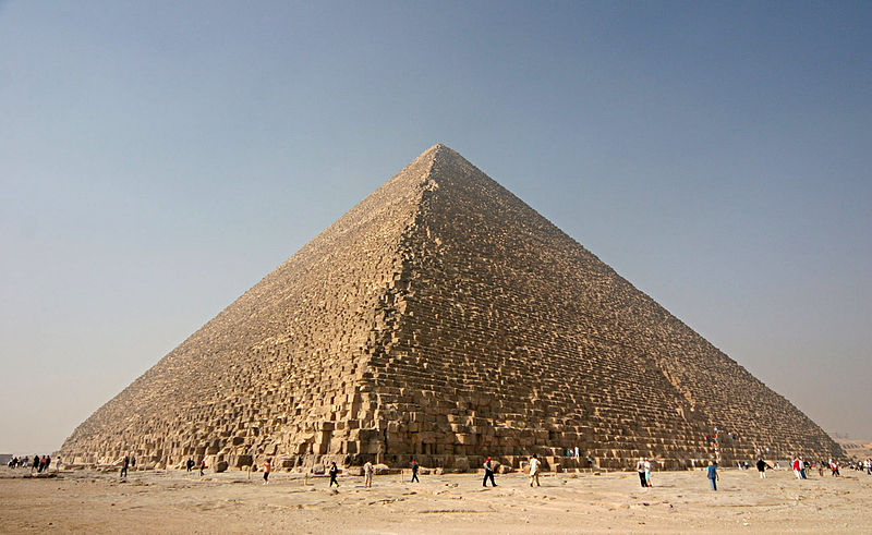
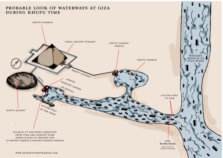
Cheops pyramid building started about 2620 BC, ancient height: 147 m
2.3 million stone blocks, avg. 2.5 t each
Required coordinated transport, tool inventory, and mass catering for about 100,000 workers

Supply chains in History

Hannibal’s invasion of Italy

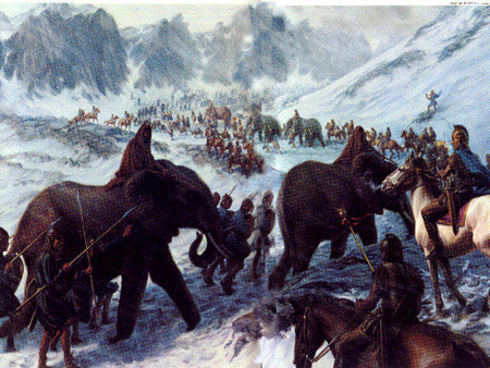
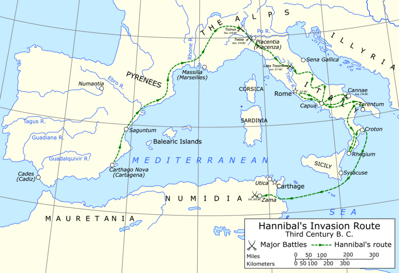
Invasion from Spain to Italy in the 2nd Punic War
37 war elephants + 40,000 troops (incl. large cavalry)
Supply of troops and beasts had to be realised in hostile territory

Supply chains in History

Toga praetexta: raw materials, purple and sales

Production process

%%{init: {
  "theme": "base",
  "themeVariables": {
    "fontSize": "11px"
  },
  "flowchart": {
    "nodeSpacing": 20,
    "rankSpacing": 25
  }
}}%%

flowchart TB
    A["Sheep farming"] --> B["Shearing and sorting<br/>of raw wool"]
    B --> D["Spinning into wool yarn"]
    D --> E["Weaving the white woollen cloth"]
    E --> F["Fulling, cleaning,<br/>bleaching, cutting"]
    F -->|"approx. 100 sesterces per pound"| H["Attaching the purple border<br/>Making up the toga"]

    P2["Snail breeding"]
    P2 --> P3["Extracting glands<br/>(hypobranchial gland)"]
    P3 --> P4["Salting glands &<br/>heating over several days"]
    P4 --> P7["Dyeing wool / wool batches<br/>purple"]
    P7 -->|"4,000 sesterces per pound"| H

    T["Total value: 400 - 1,200 sesterces per toga"]

    H ~~~ T

    classDef raw fill:#f5f1e8,stroke:#7a6a4f,color:#2b2b2b;
    classDef proc fill:#eef4fb,stroke:#5179a6,color:#112d3d;
    classDef purple fill:#f4e8fb,stroke:#7a3ea1,color:#321744;
    classDef note fill:#fff8d9,stroke:#b89b2e,color:#3a3212,stroke-width:0.01px;

    class A,B,D,E raw;
    class P2,P3,P4,P7 purple;
    class F,H proc;
    class T note;

Illustration and draping of a Roman toga, including the toga praetexta with purple border

Product	Price
Simple white toga	12 sesterces
Better white toga	60 sesterces
Toga praetexta	800 sesterces

$\rightarrow$ Annual pay of a common soldier: 1,000 sesterces

Raw material and sales map

Supply chains in History

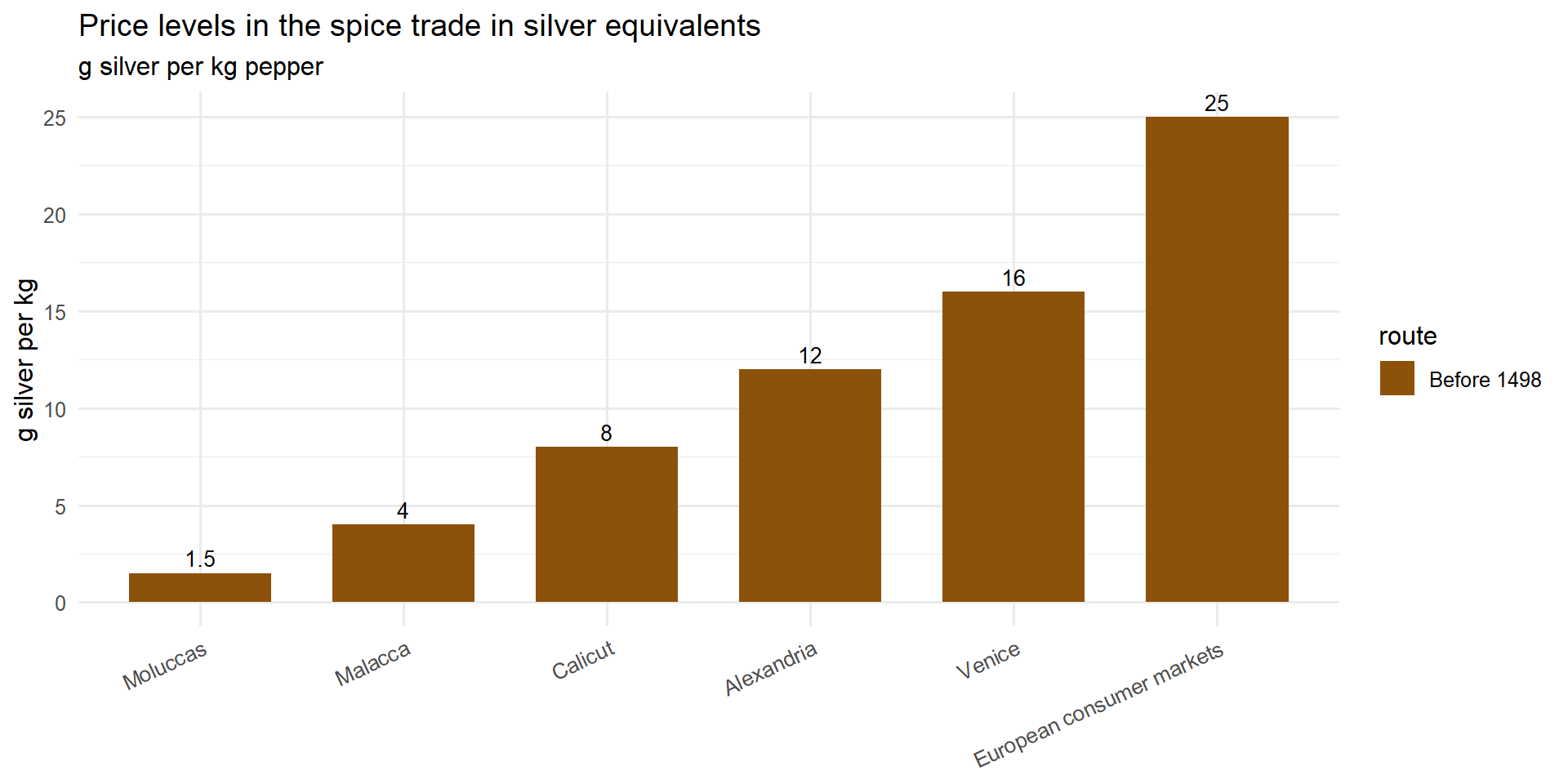
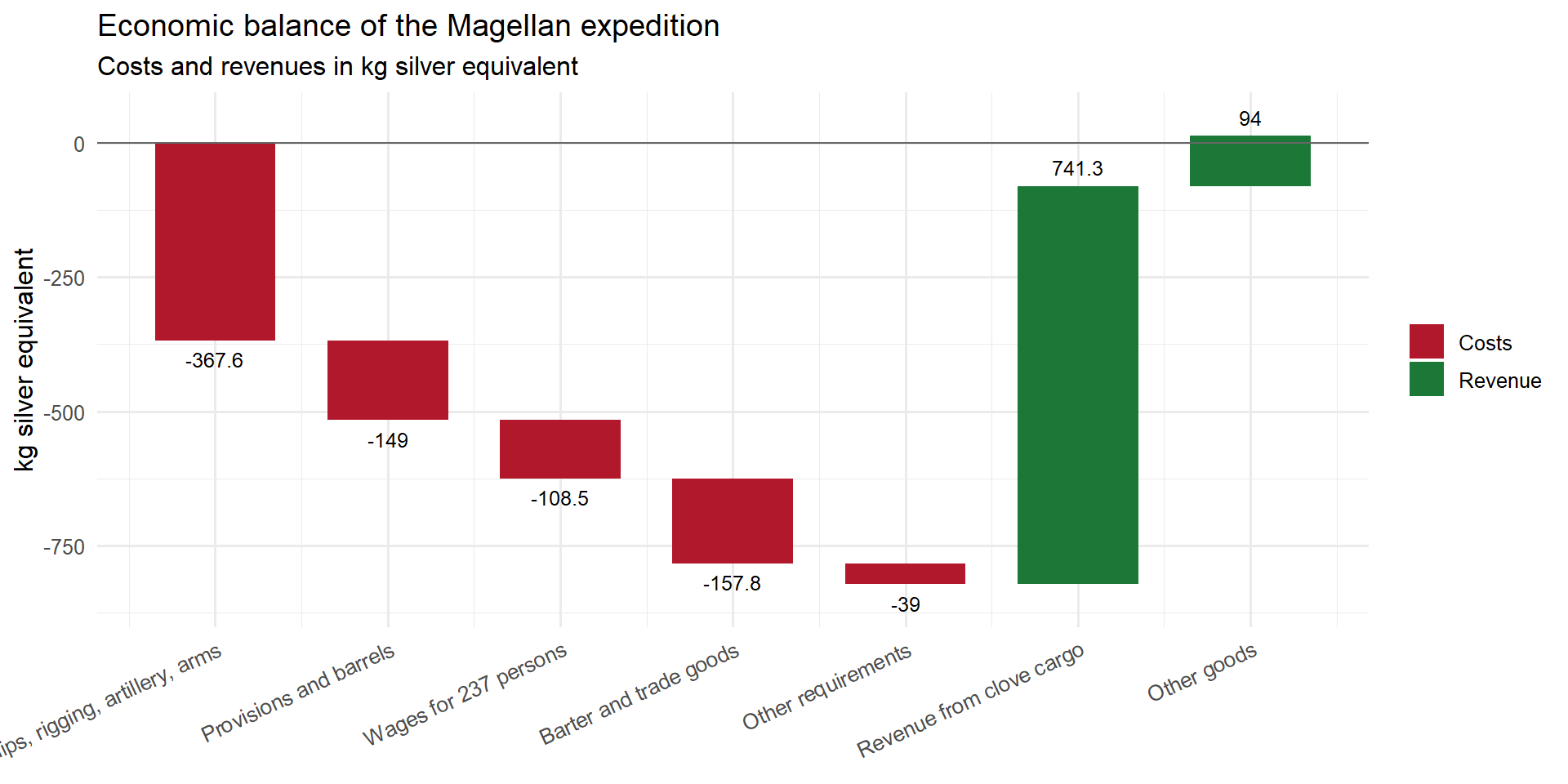
Spice trade in the 15th century

Magellan expedition of the Spanish Crown, 1519 - 1522
Goal: western sea route to the Moluccas
Start: 5 ships / 260 crew
End: 1 ship / 18 crew

Why Supply Chain Management?

Customer value along the supply chain

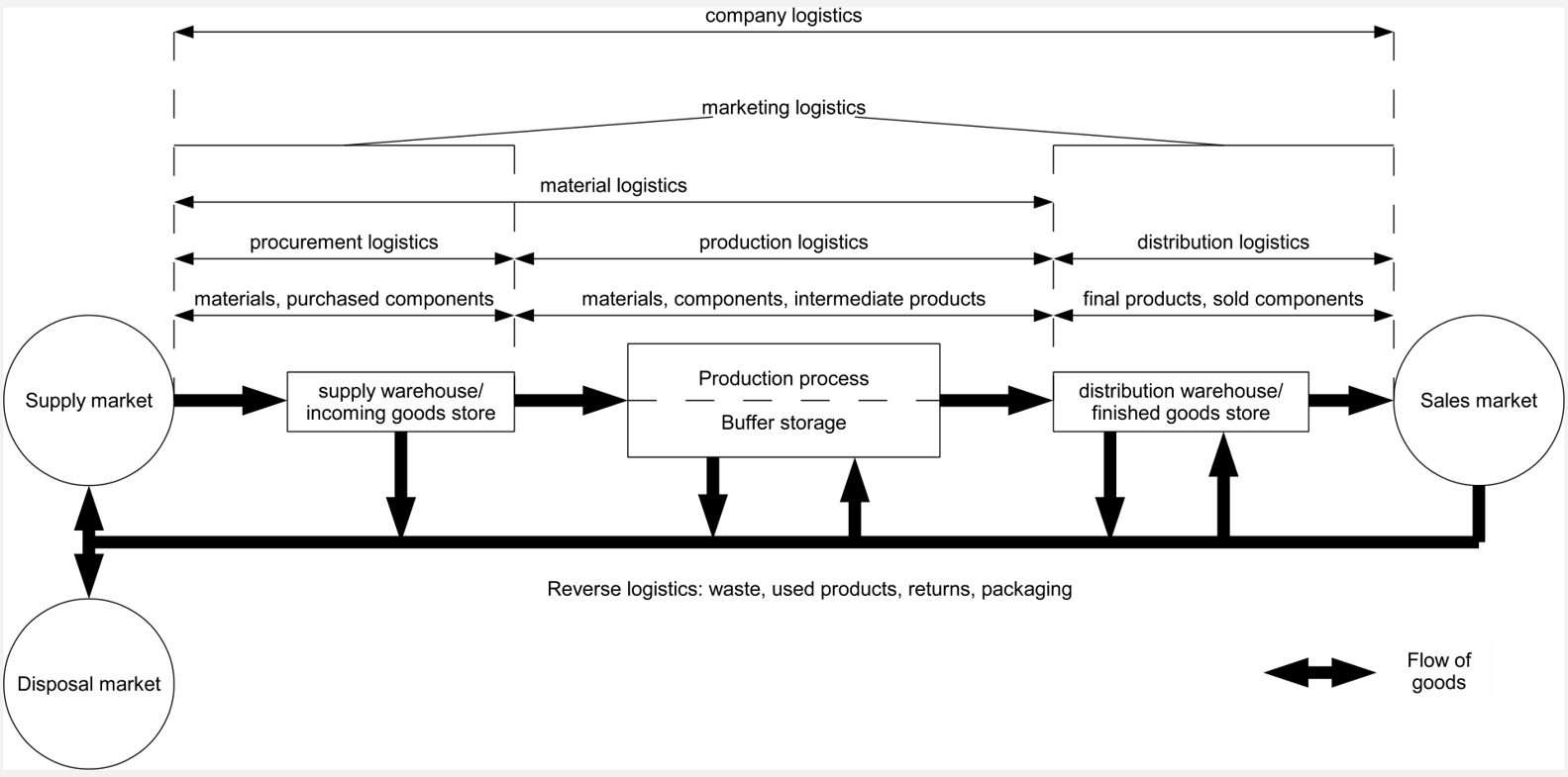
Logistics systems in the company

Supply chain structures

Network concept & basic paradigm

SCM profit = customer revenue – total costs of all processes/partners = sum of indiv. profits

$\rightarrow$ Optimising indiv. profits does not, as a rule, optimise the SCM profit!

Transformation

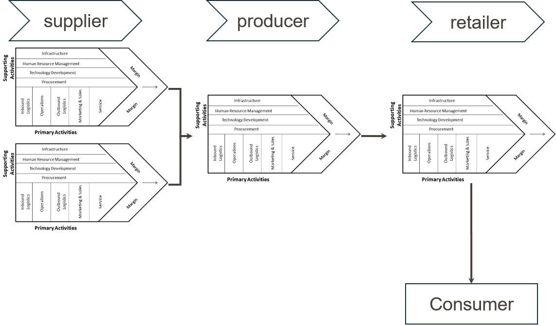
Value creation in the supply chain

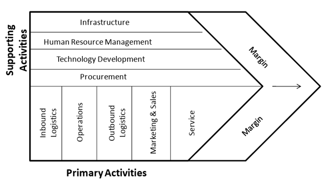
Porter’s value chain

Definitions of SCM

Diversity & common core

(Stadtler 2000, 9): “Supply chain management is the task of integrating organisational units along the supply chain, coordinating the flows of materials, information and money, and improving the competitiveness of the entire supply chain in order to meet customer needs.”

(Hugos 2018): “Supply Chain Management is coordination of production , inventory , location , transportation , and information among the participants in a supply chain to achieve the best mix of responsiveness and efficiency for the market being served .”

(Council of Supply Chain Management Professionals (CSCMP) 2013): “Supply chain management encompasses the planning and management of all activities involved in sourcing and procurement, conversion, and all logistics management activities. Importantly, it also includes coordination and collaboration with channel partners, which can be suppliers, intermediaries, third party service providers, and customers. In essence, supply chain management integrates supply and demand management within and across companies .”

Companies and their environment

Open model of the firm

(Kummer et al. 2018)

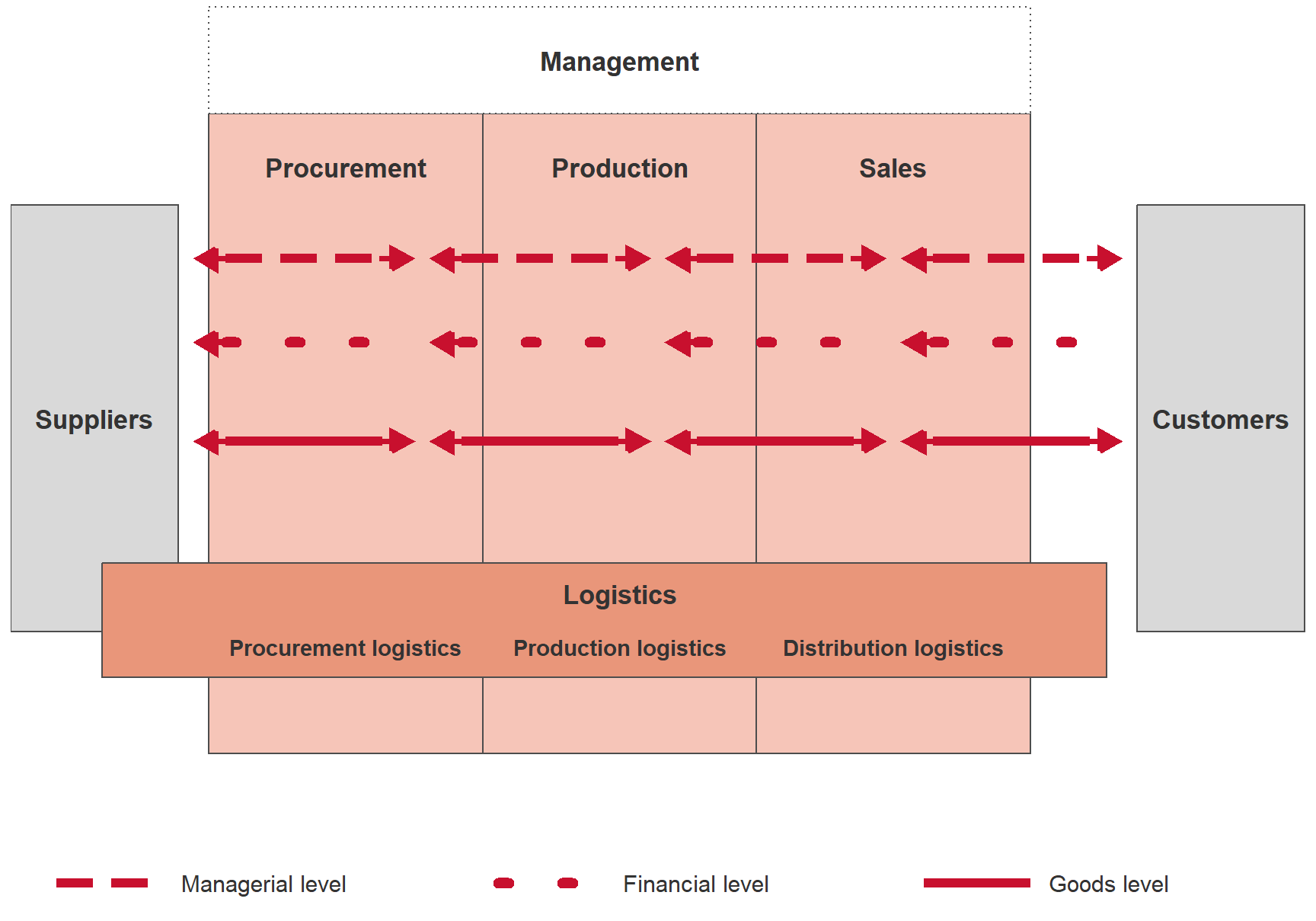
Dispositive level: covers the information flow within and between companies, planning processes, decision-making and control (management in the narrow sense)
Financial level: covers money and payment flows within and outside the company
Goods level: covers the movement and stock of physical goods (raw materials, auxiliary materials and supplies) within and between companies

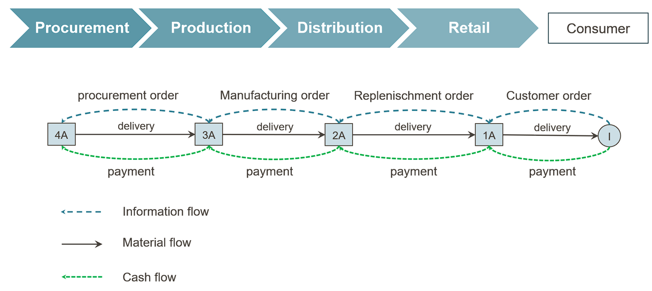
Flows in supply chains

Supply chain structures

Focal supply chain

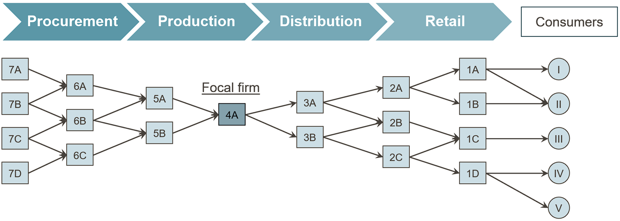
Characteristics:

Focal company in the bottleneck position → “controls” the network (actors and structure)
High market power → controls market access
Often the coordinator → sets standards and strategic objectives
Examples: automotive industry, Apple, …

Supply chain structures

Polycentric supply chains

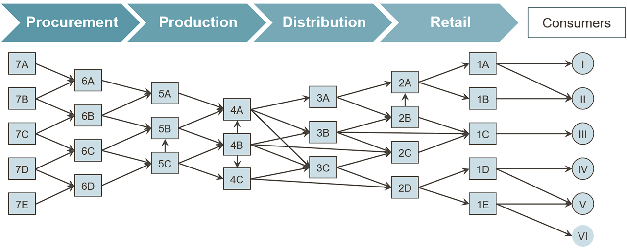
Characteristics:

Distributed and overlapping competences
Specialisation and cooperation
No clear standardisation and a rather egalitarian distribution of market power
Examples: IKEA, Neste, Unilever, …

Examples of supply chains

Task

Try to describe the structure of the supply chains, in particular the distribution structure, of the following products:

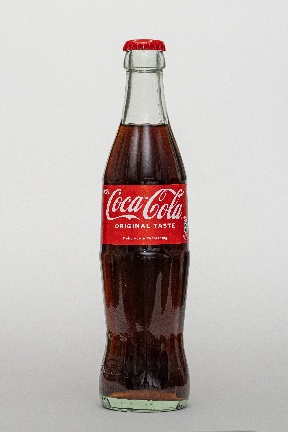
A bottle of Coca-Cola (glass, 0.3 l)
T-shirt from Patagonia
Gravel bike Waldwiesel from Urwahn
Ritter Sport Hazelnut

Describe the main production steps by specifying the raw materials, materials and components used as well as the (intermediate) product(s) created. Complement the description by specifying the logistics processes that link the production stages.

Assign the individual process steps (production and logistics) to locations.

Fundamentals of SCM - Objectives & Trade-offs

Fundamentals of Supply Chain Management

Tasks, terms and concepts
Objectives & trade-offs
Costs & management

Learning objectives

After this unit you will be able to …

structure value creation processes and the key drivers of a supply chain,
explain the terms responsiveness and efficiency,
contrast the implied uncertainty of a market with the responsiveness of a supply chain,
assess the strategic fit of a supply chain configuration.

Further reading

Strategic fit, supply chain drivers and implied uncertainty: (Chopra and Meindl 2025, chaps. 2–3).
Matching supply with demand and operational capability: (Cachon and Terwiesch 2024, chaps. 1–3).
Supply chain strategy and value-oriented logistics: (Christopher 2023, chaps. 2–4).

Value creation as a process

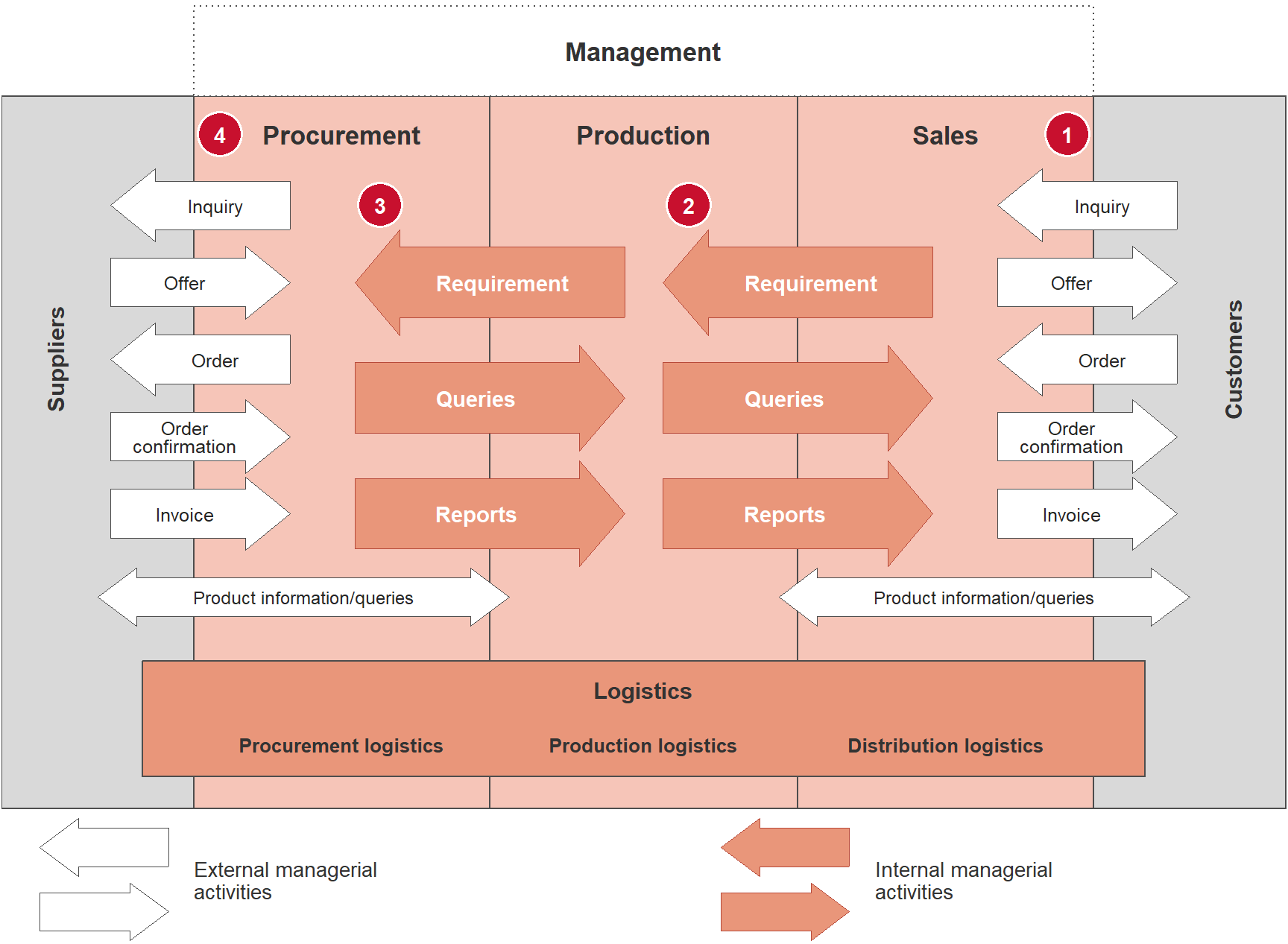
Procurement is the process of purchasing and providing raw materials, components and services from external partners that are required for the production of goods and services.

Production is a purposeful process of combining goods and services into higher-value products.

Distribution covers the physical distribution of goods from the manufacturer to the end customer and includes warehousing, transport and logistics of finished products.

Sales is the process of selling the end products to consumers or trading partners.

Strategic manufacturing

Decoupling point & manufacturing strategies

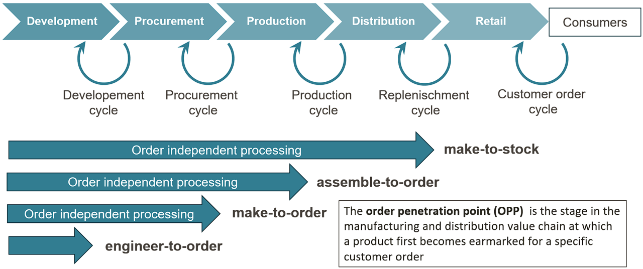
Strategic manufacturing

Thinking in cycles

Customer order cycle: processing of external customer demand

Distribution/replenishment cycle: conversion of customer demand into internal demand for finished products

Production cycle: conversion of internal demand into production requirements for intermediate products and raw materials

Procurement cycle: design of ordering/supply processes for raw materials and services that have to be sourced externally

(Kummer et al. 2018, 45)

Strategic manufacturing

Decoupling of cycles

Make-to-stock

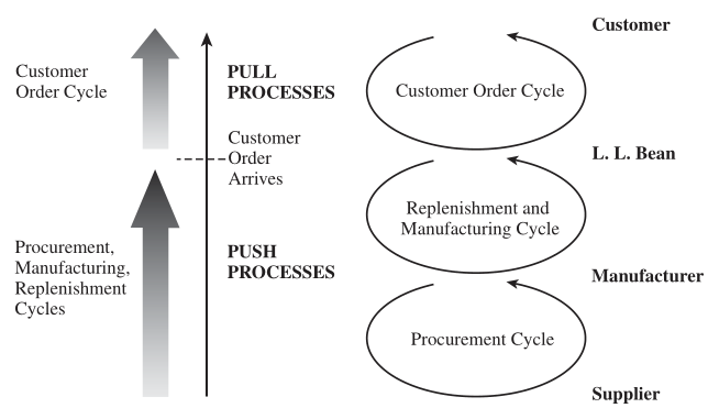
Examples: grocery retail, drugstores, …

Make-to-order

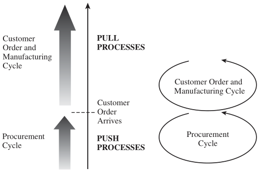
Examples: buildings, aircraft, paintings

(Chopra and Meindl 2025)

Strategic objectives

Customer satisfaction – meeting customer expectations

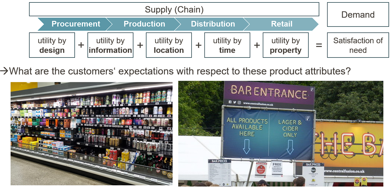
Strategic objectives

Customer satisfaction & uncertainty

Customers and supply chain uncertainty

Quantity demanded per customer order
Lead time accepted by customers
Expected product variety
Expected service level
Price/willingness to pay
Degree of product innovation

Demand uncertainty

Uncertainty of the demand for a product

Implied demand uncertainty

Uncertainty of the demand segment that the supply chain is intended to serve, based on the defined demand attributes

Dealing with uncertainty

Customer needs & implied uncertainty

Customer needs	Causes implied uncertainty because …
(Max.) demand quantities increase	Wider range of demand causes greater variance / fluctuation of demand quantities
Lead time decreases	Less time remains to react to demand fluctuations
Number of products offered increases	Demand for individual products is harder to forecast
Required service level increases	Demand peaks now have to be absorbed
Degree of innovation increases	Demand for new products is usually unknown or hard to forecast
Number of sales channels increases	Demand per sales channel is harder to forecast

Dealing with uncertainty

Roles & risk allocation in the supply chain

(Chopra and Meindl 2025, 57)

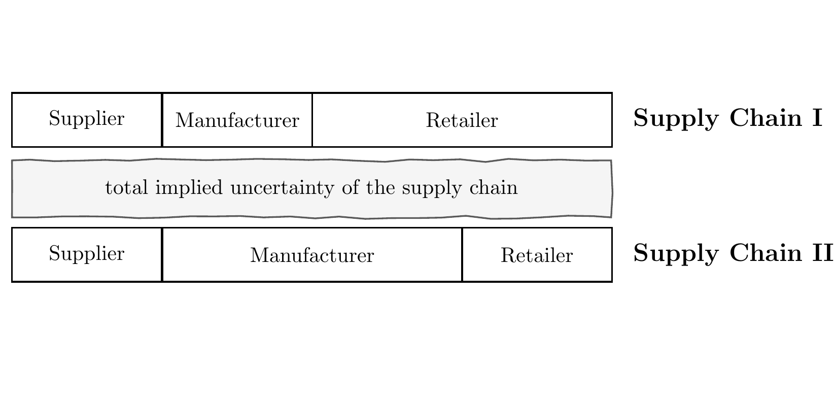
Dealing with uncertainty

Responsiveness

Responsiveness

is the ability of a supply chain to deal with demand uncertainty

Responsiveness can be achieved, among other things, through:

High inventory levels
Short response/lead times
High product variety
Short development cycles for new products
High service levels
Reduction of supply uncertainties

(Chopra and Meindl 2025, 56)

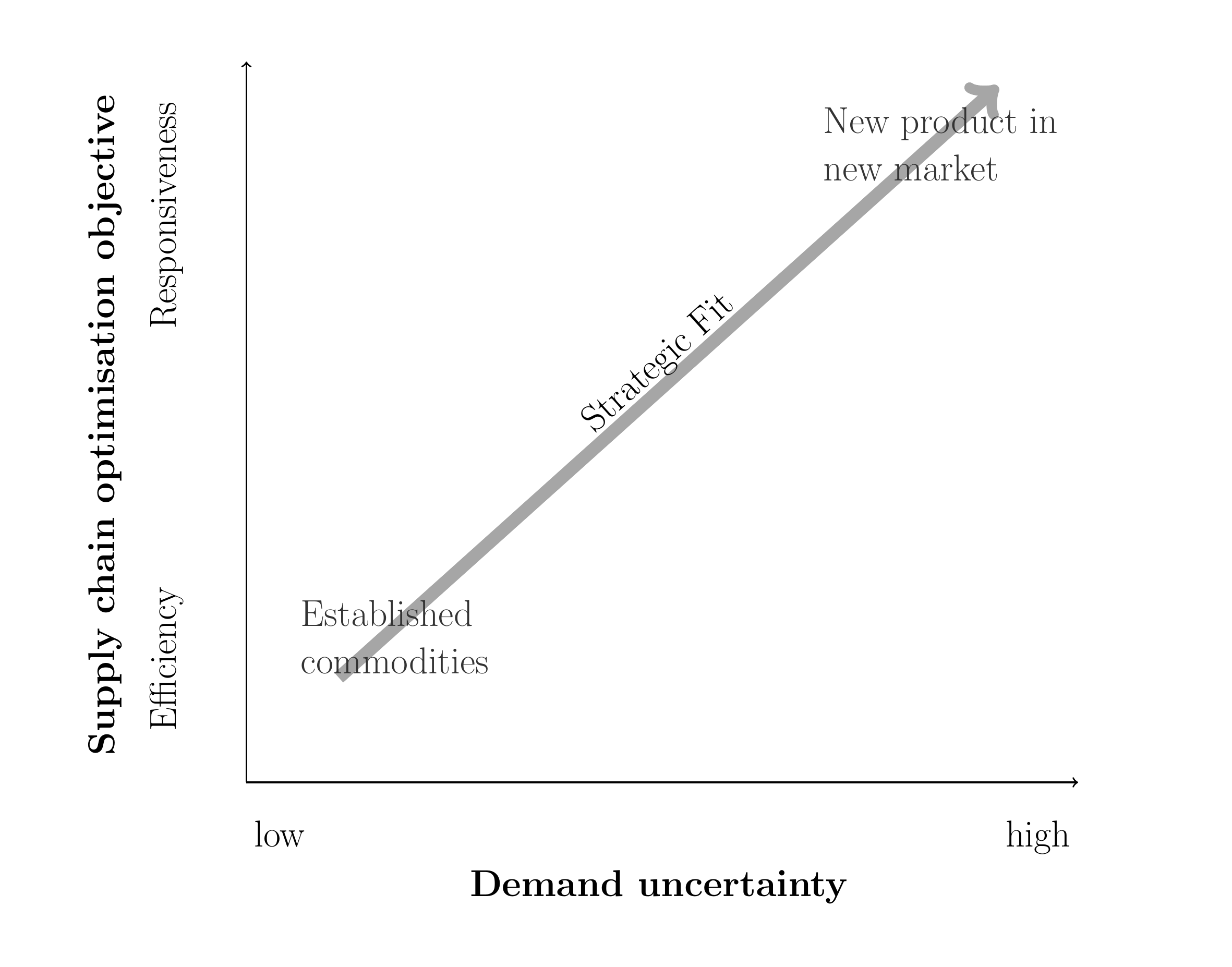
Strategic objectives

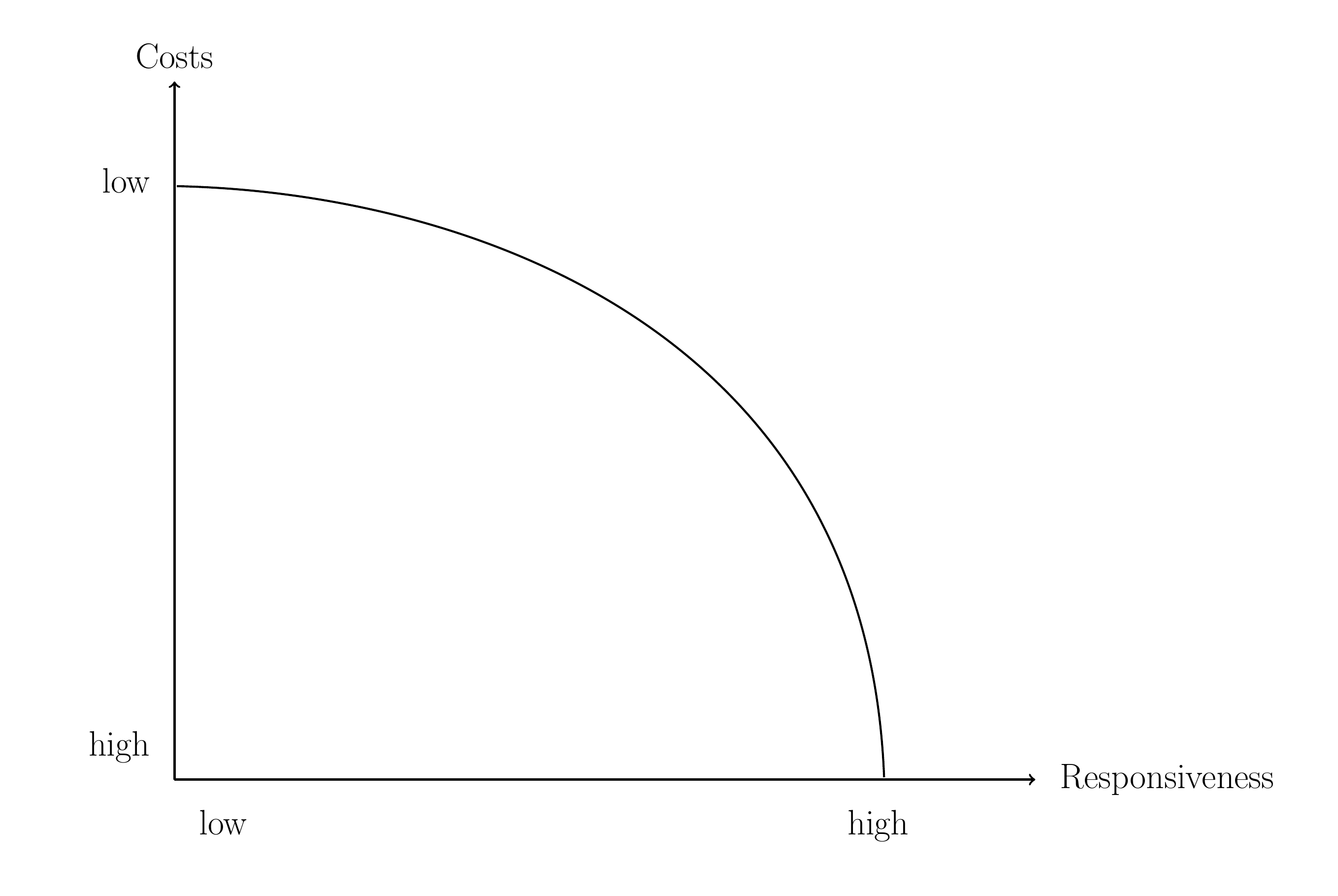
Responsiveness vs. efficiency

Responsiveness

The responsiveness of a supply chain is the ability of a supply chain to deal with demand uncertainty

Strategic drivers

$\rightarrow$ Responsiveness causes costs!

Efficiency

The efficiency of a supply chain is the inverse of the total costs of a supply chain, i.e. of all costs of a product from

Strategic management

Supply chain drivers

Figure 3

Production technology
Product portfolio
Vertical integration

Transport modes
Storage capacities
Safety stocks

Supplier selection
Facility capacities
Stages & links

Pricing
Demand management
Discounting

Information sharing
System integration
Collaborative forecasting & planning

Strategic management

Sub-strategies

	Efficient supply chains	Responsive supply chains
Primary objective	Meet demand at the lowest cost	Meet demand as quickly as possible
Product design strategy	Low product variety, focus on simple design and high throughput	Modular product development and postponement
Pricing strategy	Low prices and margins since customers are price-sensitive	Higher prices with higher margins, since customers are not very price-sensitive
Manufacturing strategy	High machine utilisation	Spare capacity to be able to expand production quantities at short notice
Inventory strategy	Minimise (safety) stocks	Build up safety stocks to buffer demand fluctuations
Lead time strategy	Reduce cycle times as long as costs do not increase	Reduce cycle times even if costs increase
Procurement strategy	Supplier selection based on cost and reliability	Supplier selection based on responsiveness, speed, flexibility and quality

Strategic management

Generic strategies & SCM

Generic strategy	Advantage	Basis of competition	Contribution of SCM
Cost leader	Drive cost-efficient production	Lowest prices in the product category	Efficient, low-cost infrastructure
Innovation leader	Exploit market strength and deploy unique technology	Generate sought-after and innovative products	Secure short time-to-market, increase volume
Service leader	Tailor service consistently to customers	Meet customer-specific expectations	Enable customer-oriented development
Quality leader	Manufacture safe and reliable products	Unique product features	Reliable SC, quality assurance
Sustainability leader	Sustainable products and processes	Meet customers’ sustainability expectations	CO2 neutrality, conservation of energy and resources

SCM Fundamentals – Costs & Management

Fundamentals of Supply Chain Management

Tasks, terms and concepts
Objectives & trade-offs
Costs & management

Learning objectives

After this unit you will be able to …

name the key economic, ecological and social objectives of supply chain management,
analyse trade-offs between service, inventory, transport, costs and sustainability,
explain and quantify the main components of logistics costs,
select and interpret suitable metrics for evaluating logistics decisions.

Further reading

Systems of objectives and cost models: (Günther and Tempelmeier 2012, chaps. 1–3).
Performance and cost perspective of distribution logistics: (Tripp 2024, chaps. 1–4).
Sustainability as a corporate objective: (Dyckhoff et al. 2008, chaps. 1–3).

Types of objectives in the company

Levels in the management system

(Dyckhoff 1998)

Objectives in the management system

(Buscher et al. 2013, 12)

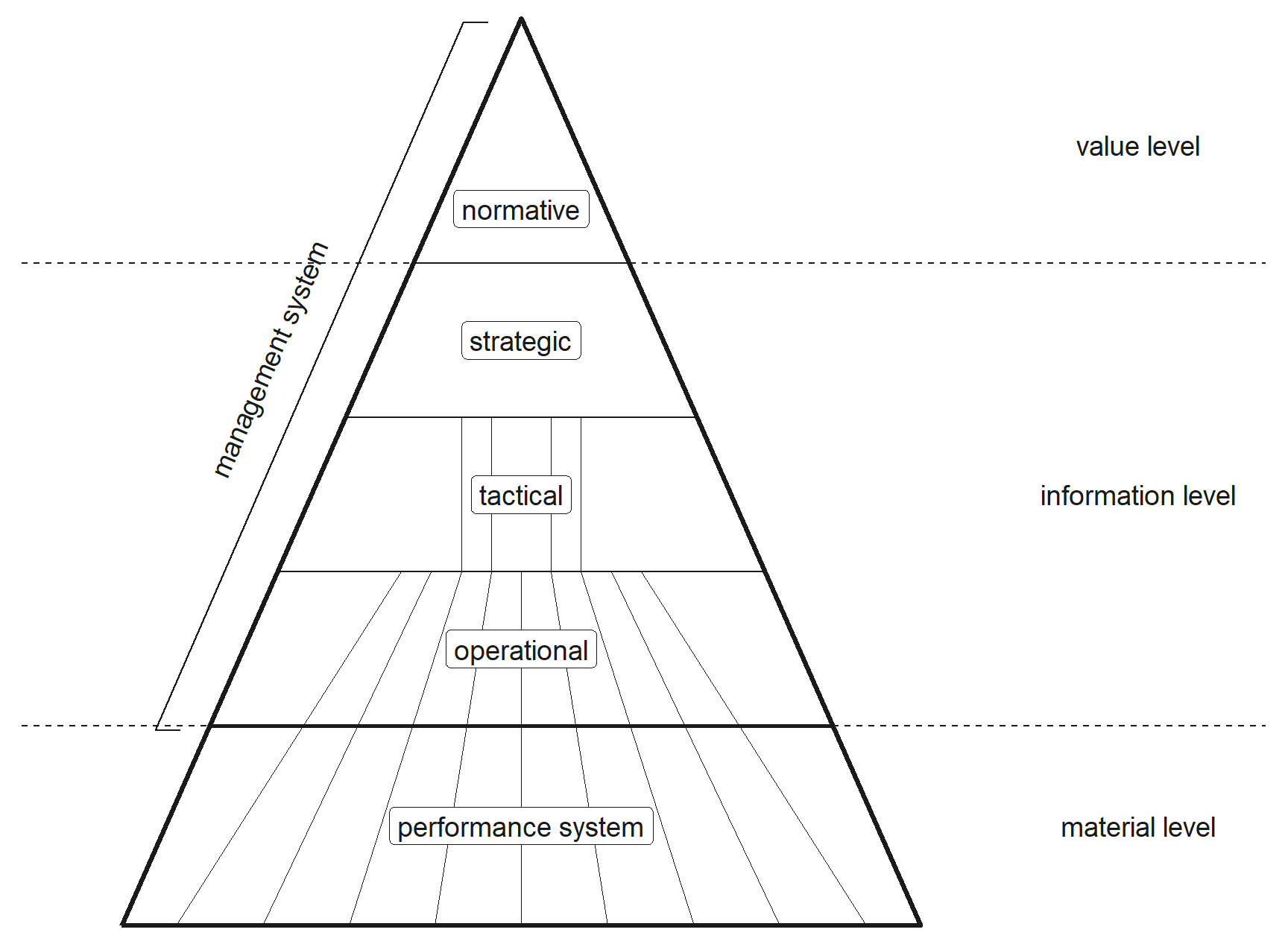
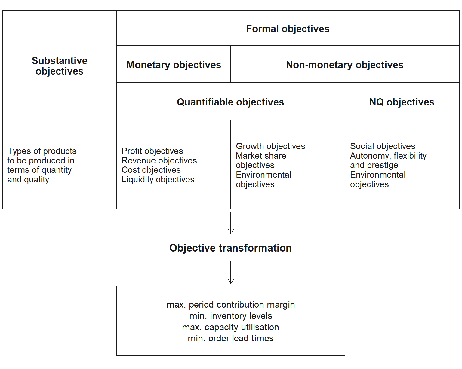
Objectives in logistics and SCM

Traditional target metrics

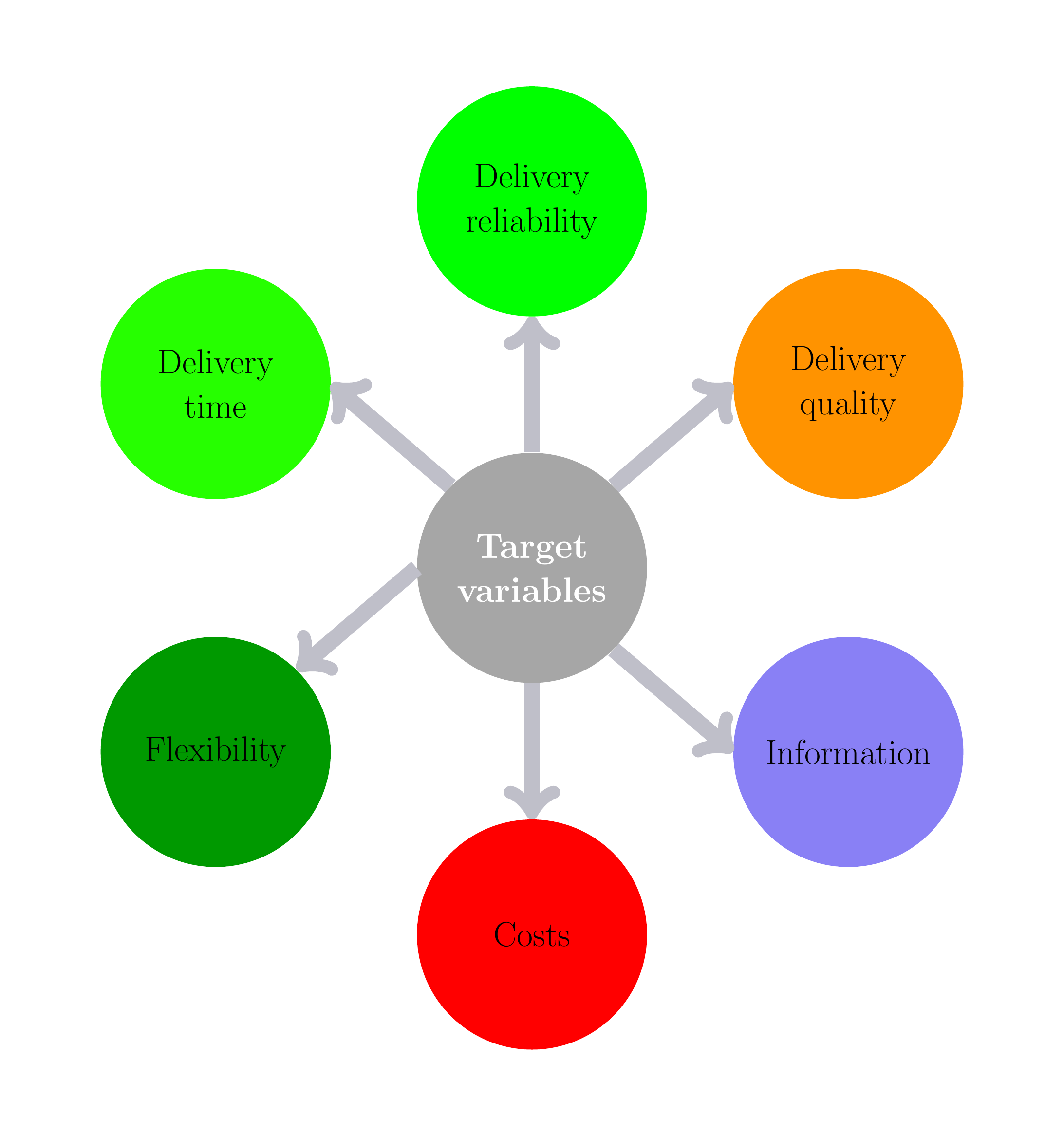
Delivery time: time span between order placement and order fulfilment
Delivery reliability: relationship between promised and actual delivery date
Delivery quality: share of orders executed correctly in terms of quality and quantity
Flexibility/resilience: feasibility of short-term changes in quantity, dates and specifications
Information: quality and transparency of information in all phases of order processing
Costs: efficiency of all logistics activities, total costs of logistics activities

Target dimensions

Conflicts & profiles

Target dimensions

Target profiles

Logistics costs

Trade-off decisions in logistics and SCM

Mode of transport
Number of warehouses
Safety stock
Lot size

Conflicting cost components in many areas of logistics $\rightarrow$ a cost optimum exists (at least in theory)
Logistics management means, among other things, making decisions about logistics systems
Transparency of cost functions is sometimes severely limited
- Data availability
- Intertemporal attributability
- Cost object assignment
- Stochasticity

Logistics costs

Examples

Logistics costs

valued consumption of goods and services for the purpose of providing logistics services.

Bananas
McKinsey

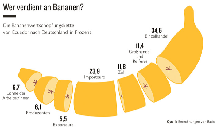
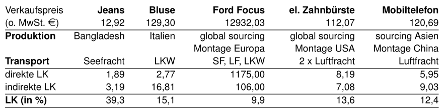
Supply Chain Costing

Example – Apple Video iPod 30 GB

(Dedrick 2012)

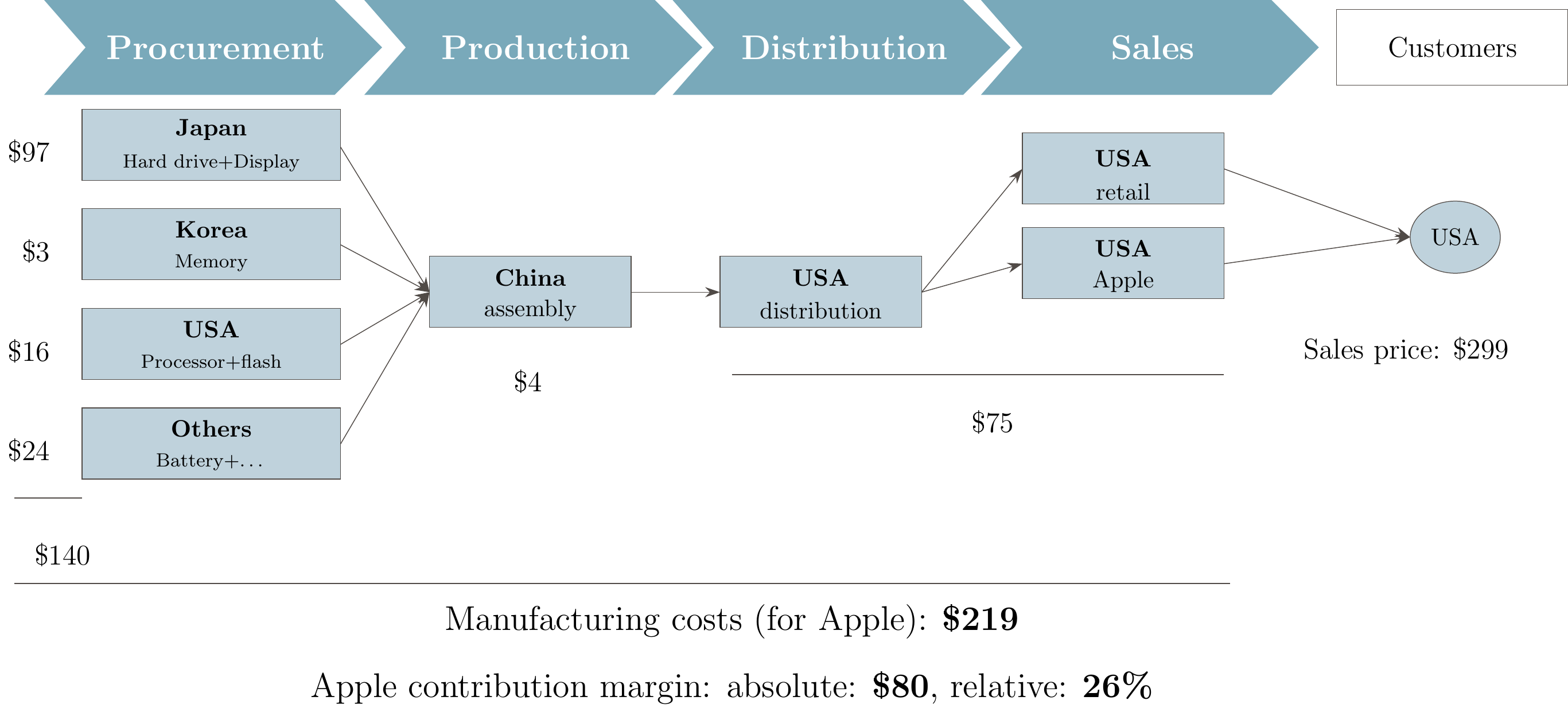
Sustainable Supply Chain management

Sustainability as a target dimension

Definition of sustainability (an attempt)

A social system is described as sustainable if it can be regarded as fair both intra- and intergenerationally. Fair means that it “meets the needs of the present without compromising the ability of future generations to meet their own needs” (Hauff 1987)

Sustainability & sustainable development

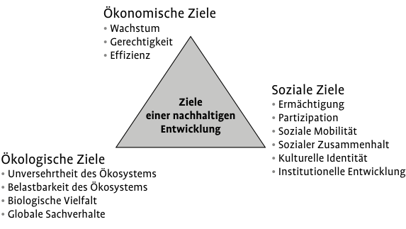
Possible target dimensions

Content placeholder 13

(Baumast and Pape 2013)

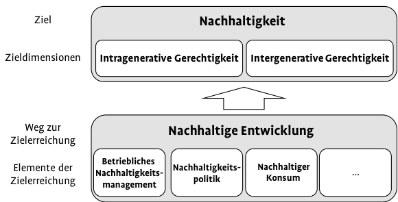
Ecological strategic fit

Ecological orientation and exposure (Günther 2008)

Ecological resistance

High exposure but low ecological orientation. Delaying or minimalist response patterns are typical.

SKW Piesteritz (chemicals)
only minimum regulatory adjustment; ecological investments are postponed, lobbying

Dimensions of ecological SCM strategies

(Dyckhoff et al. 2008)

Sustainability

General concepts (Ellen MacArthur Foundation)

Sustainability pyramid

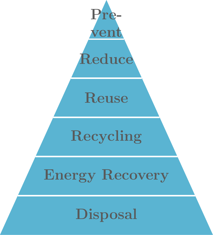
Circular economy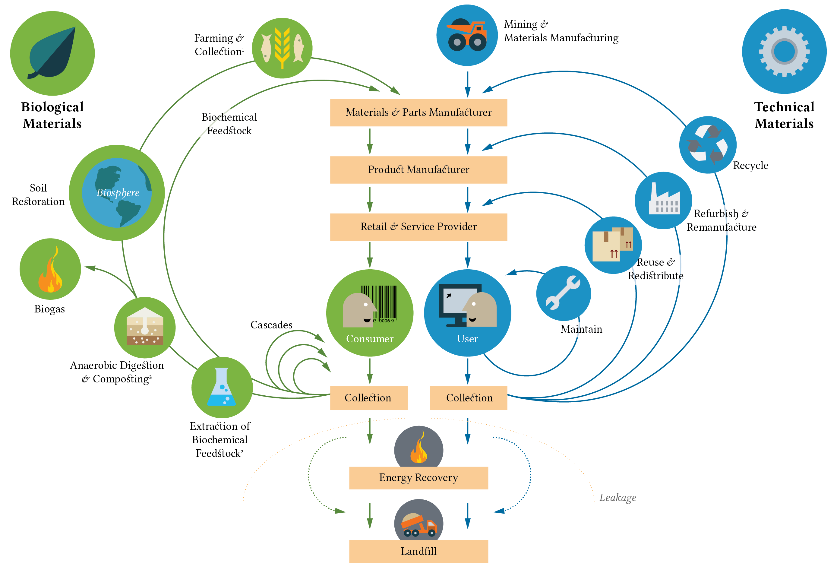

Circular Supply Chain

Relationship between linear, reverse and circular supply chains

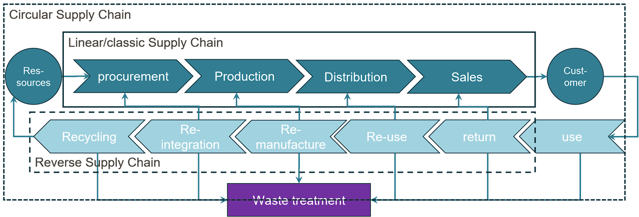
Sustainable SCM

refers to the planning, execution and control of business processes taking into account economic, ecological and social objectives in order to ensure the long-term competitiveness of the supply chain.

Sustainable Supply Chain Management

Circularity & sustainability concepts

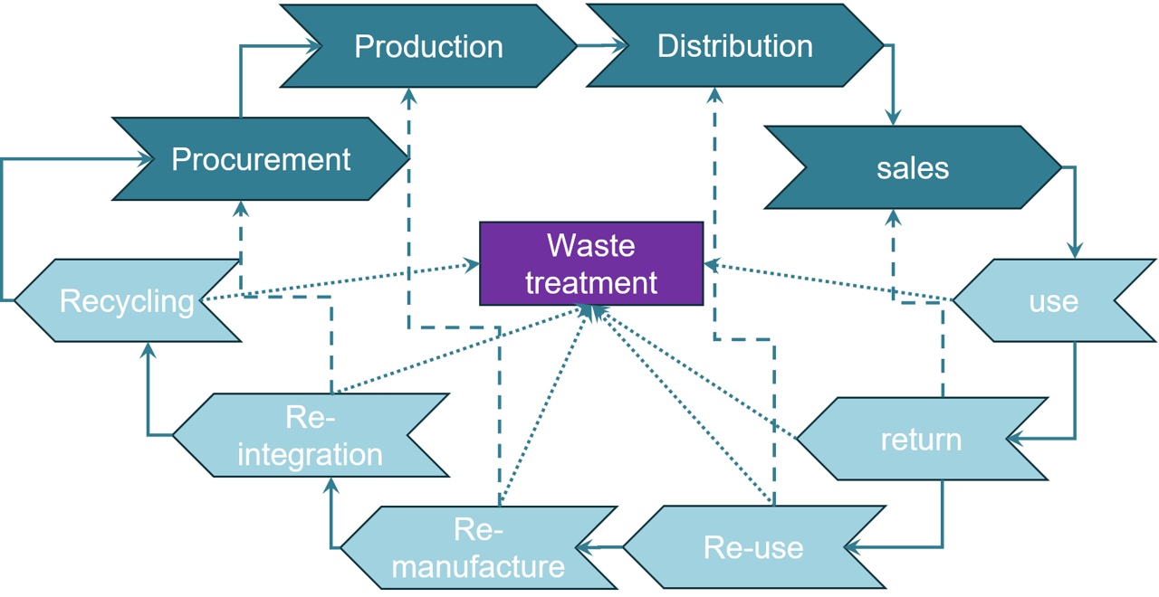
Circular Product Design
- Recyclability
- Reuse
- Recycled content
Sustainable logistics
- Weight reduction
- Distance reduction
- Transport avoidance
Circular production
- Renewable energy
- Use of production waste
- Recirculation of operating supplies and auxiliary materials

Sustainable SCM

Planning tasks

(Stindt 2017)

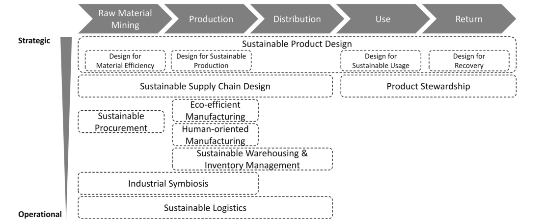
Circular Supply Chain Management

Generic strategies

Circular Supply Chain Management

Generic strategies

Circular Supply Chain Management

Generic strategies

Circular Supply Chain Management

Generic strategies

Case example SushiFresh GmbH

The business idea

SushiFresh GmbH is a start-up offering sushi boxes freshly made every day in a German metropolitan region.

Promise: “Made today, sold today” – restaurant-quality sushi, but without the wait
Production: one central kitchen, production in the early morning hours
Sales channel: supermarkets (shelf sales)
Range: approx. 12 boxes (classic, vegetarian, vegan)

Key facts

Shelf life: max. 24–36 hours
Cold chain: continuously 0–4 °C
Ingredients: rice, nori, vegetables (regional), salmon and tuna (imported)
Demand: highly volatile (weekday, weather, events)
Market launch: growth from 3 to 30 points of sale planned

Case example SushiFresh GmbH

Discussion

Guiding questions: strategic position

Which customer groups and needs drive the positioning – price, freshness, convenience or sustainability?
How does SushiFresh differ from competitors (restaurants, delivery services, supermarket sushi)?
Which trade-offs arise (freshness vs. costs vs. waste vs. environment)?
Where does the company sit between efficiency and responsiveness? Which target variables are strategically important?

Guiding questions: supply chain structure

How does the supply chain deal with volatile demand and highly perishable goods?
How can the cold chain and freshness be ensured along the entire chain?
Which stages and partners belong to the supply chain (suppliers, kitchen, logistics, retail)?
How should the supply chain be structured: centralisation vs. decentralisation?
What depth of value creation could SushiFresh aim for? (e.g. in-house logistics?)

Objective: Prepare a strategic analysis of SushiFresh’s business model. Derive a suitable supply chain structure.

Strategic Design of Supply Chains

Multi-criteria facility location planning
Continuous facility location planning
Discrete facility location planning

Learning objectives

After this unit you will be able to …

classify location decisions within strategic supply chain design,
systematically capture and evaluate qualitative location factors,
explain and apply the AHP method and the scoring model,
explain the properties of different distance metrics and calculate them,
apply and interpret continuous location methods for simple decision problems.

Further reading

Model-based regional facility location planning and development: (Kik 2022).
Facility location planning and continuous decision models: (Thonemann 2023, chap. 3).
Continuous location models and local equilibria: (Cooper 1968).

Planning in Supply Chain Management

Supply Chain Planning Matrix

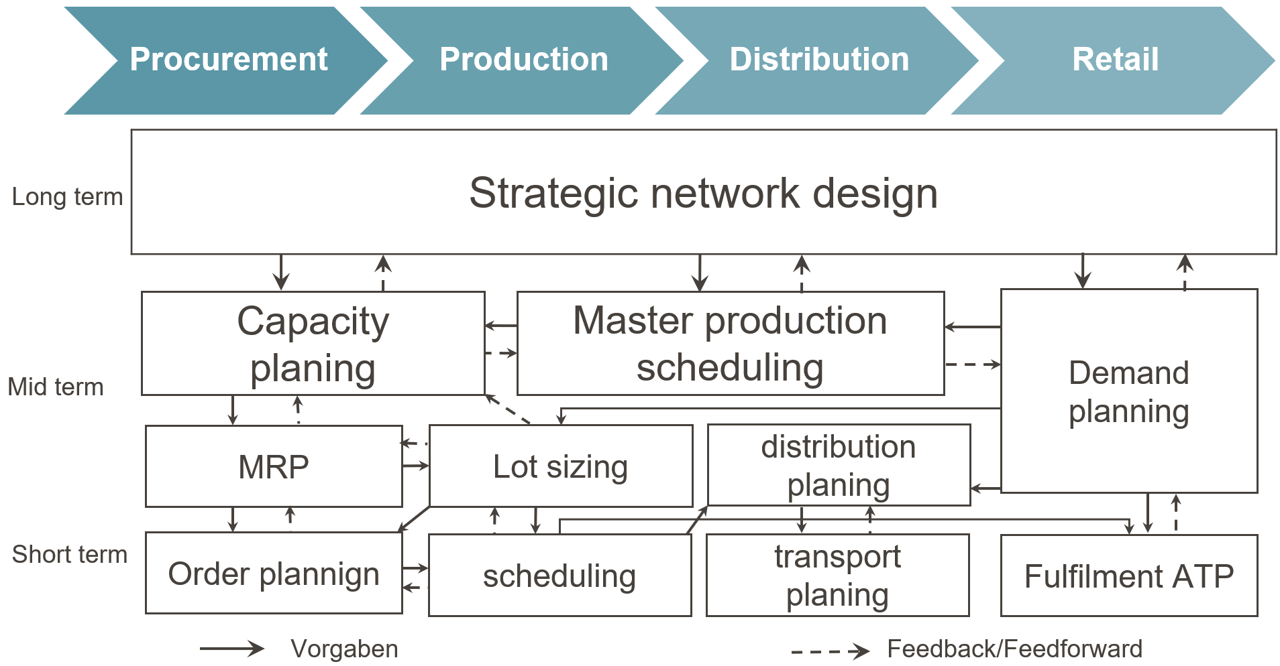
Strategic Network Planning

Objective of facility location planning

Decision on the location of:

distribution warehouses
factories
sales outlets
supply warehouses
…

Strategic Network Planning

Phases of location selection

(Chopra and Meindl 2025)

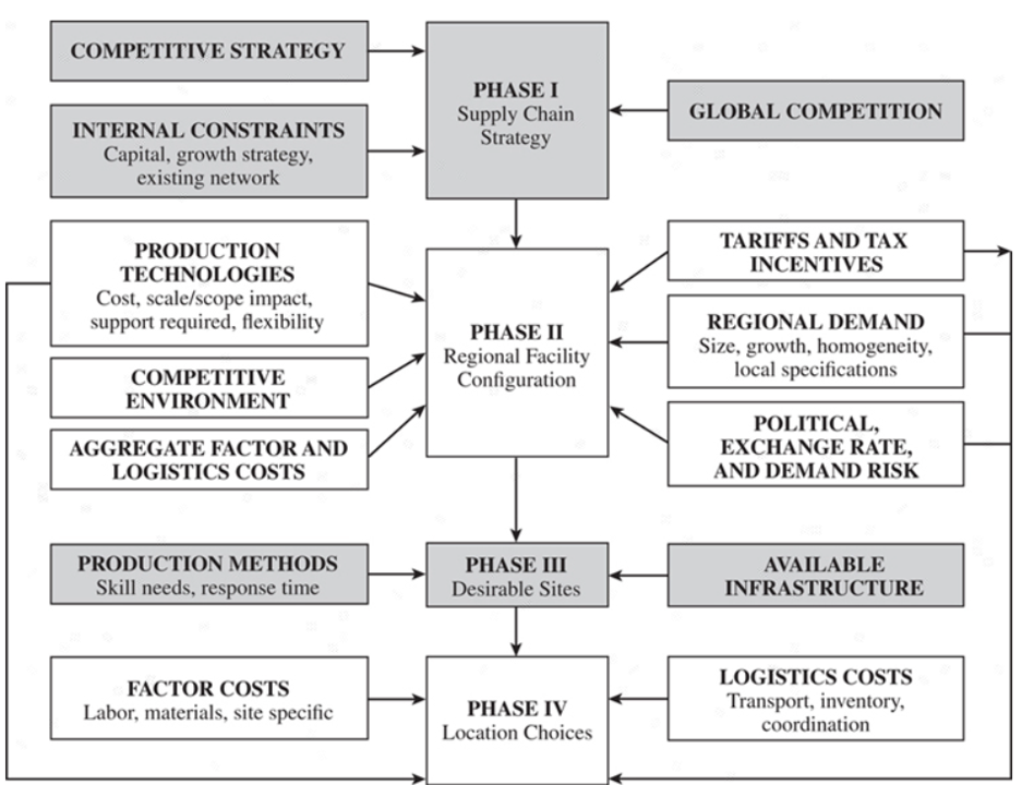
Strategic Network Planning

Facility location planning process

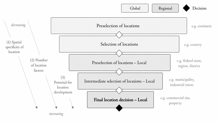
(Kik 2022)

At global level, options are usually limited (continent/country) $\rightarrow$ factors heavily simplified and aggregated $\rightarrow$ non-specific; goal is strategic fit
At regional level, goal is to identify the optimal location $\rightarrow$ more precise requirements

Strategic Network Planning

Location factors

(Lahner 2020)

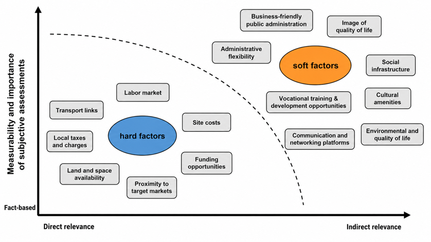
Evaluating sites for new facilities is often difficult
irreversible in the short term $\rightarrow$ path dependencies
Multidimensional $\rightarrow$ effects on the system of objectives hard to oversee
Subjective $\rightarrow$ assessments of soft factors often vary & their importance is weighted differently

Strategic Network Planning

Methods of facility location planning

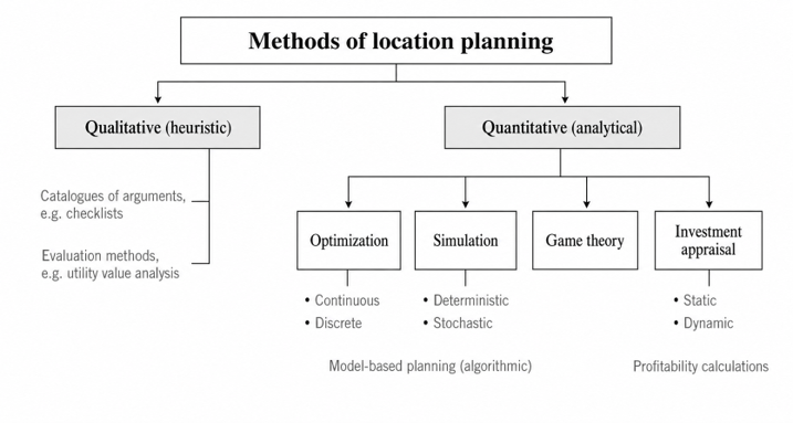
(Kik 2022)

Qualitative methods $\rightarrow$ heuristic, mostly survey-based methods $\rightarrow$ snapshot of opinion and collection of individual assessments
Quantitative methods
- Optimisation: decision space (options) and one-dimensional system of objectives required
- Simulation: complex, hard to transfer, multidimensional
- Game theory: anticipation of competitor behaviour $\rightarrow$ sales maximisation
- Investment appraisal: exclusively monetary quantities (optimisation)

Strategic Network Planning

Case study: SushiFresh GmbH

SushiFresh GmbH is a fictitious regional producer of fresh sushi boxes in the Rhine-Main region that supplies six supermarket stores every day. This case study accompanies us through this and the following chapters.

SushiFresh is examining whether, in addition to delivery, an own production facility is worthwhile, and has identified three candidate sites.

# Six stores: coordinates, daily demand mu and standard deviation sigma
filialen <- tibble(
  Filiale = c("Wiesbaden", "Mainz", "Frankfurt", "Ruesselsheim", "Darmstadt", "Offenbach"),
  lat   = c(50.0782, 50.0000, 50.1109, 49.9904, 49.8728, 50.0956),
  lon   = c(8.2398,  8.2711,  8.6821,  8.4116,  8.6512,  8.7761),
  mu    = c(120, 150, 280, 90, 110, 95),
  sigma = c(25, 30, 55, 20, 24, 22)
)

# Three candidate locations for the production facility
standorte <- tibble(
  Standort = c("Wiesbaden-Erbenheim", "Mainz-Hechtsheim", "Raunheim"),
  lat = c(50.0632, 49.9698, 50.0000),
  lon = c(8.2999,  8.2831,  8.4650),
  Fixkosten = c(180000, 210000, 260000)
)

sum(filialen$mu)  # Total demand: 845 boxes/day

[1] 845

Qualitative Facility Location Planning

Scoring model (utility analysis)

Procedure

Define relevant evaluation criteria
Determine criteria weights
Rate alternatives per criterion
Aggregate weighted partial scores into a total score
Rank alternatives by total score

Critical points

Additive model only interpretable to a limited extent
Poor ratings can be compensated by good ones
Utility independence of criteria often questionable
Results are sensitive to the weighting
Risk of goal fragmentation

Case example

SushiFresh evaluates the three candidate locations Wiesbaden-Erbenheim, Mainz-Hechtsheim and Raunheim for the new production facility using the criteria transport proximity, rental costs and availability of skilled labour, which for simplicity are weighted equally here.

The set-up is deliberately chosen to produce very different location profiles: Wiesbaden-Erbenheim is strong on rental costs, Raunheim on transport proximity, while Mainz-Hechtsheim leads on skilled labour.

This very example shows the weakness of the additive scoring model: despite clearly different profiles of strengths and weaknesses, all alternatives can achieve the same total score.

Qualitative Facility Location Planning

Scoring model in R: code and results table

library(dplyr)
library(knitr)

# Table with raw data of the case study (three criteria, equally weighted)
nwa <- tibble(
  Kriterium = c(
    "Transport proximity",
    "Rental costs",
    "Skilled labour availability"
  ),
  Gewicht = c(1/3, 1/3, 1/3),
  `WI-Erb`  = c(5, 8, 2),
  `MZ-Hech` = c(2, 5, 8),
  Raunheim  = c(8, 2, 5)
)

# Calculate the scores of the locations
nutzwert <- c(
    `WI-Erb`  = sum(nwa$Gewicht * nwa$`WI-Erb`),
    `MZ-Hech` = sum(nwa$Gewicht * nwa$`MZ-Hech`),
    Raunheim  = sum(nwa$Gewicht * nwa$Raunheim)
  )

# Combine raw data and scores in one table
nwa <- bind_rows(nwa, nutzwert)

# Set name "Score" in row 4, column Kriterium
nwa$Kriterium[4] <- "Score"

# Output table
nwa |>
  mutate(
    Gewicht = ifelse(is.na(Gewicht), "", sprintf("%.2f", Gewicht)), # Show 2 decimal places
    `WI-Erb` = sprintf("%.1f", `WI-Erb`),
    `MZ-Hech` = sprintf("%.1f", `MZ-Hech`),
    Raunheim = sprintf("%.1f", Raunheim)
  ) |>
  kable(
    col.names = c("Criterion", "Weight", "WI-Erb", "MZ-Hech", "Raunheim"),
    format = "html",
    align = c("l", "c", "c", "c", "c")
  )

Criterion	Weight	WI-Erb	MZ-Hech	Raunheim
Transport proximity	0.33	5.0	2.0	8.0
Rental costs	0.33	8.0	5.0	2.0
Skilled labour availability	0.33	2.0	8.0	5.0
Score		5.0	5.0	5.0

Qualitative Facility Location Planning

Analytic Hierarchy Process (AHP method)

Bottom level: Determine how the alternatives contribute to the criteria.

⇓

Medium level: Determine how the evaluation criteria contribute to achieving the objective.

⇓

Top level: Determine the best of the given alternatives (objective).

Bottom-up hierarchy (Klein and Scholl 2011, 361)

Procedure

Carry out pairwise comparisons between all alternatives with respect to the evaluation criteria.
Derive a ranking of alternatives for each evaluation criterion (synthesis).
Carry out pairwise comparisons between all evaluation criteria.
Derive a ranking of the evaluation criteria (synthesis).
Calculate the score for the alternatives.

Qualitative Facility Location Planning

Analytic Hierarchy Process (AHP method) – example

Case example

SushiFresh now compares the three candidate locations Wiesbaden-Erbenheim (W-E), Mainz-Hechtsheim (M-H) and Raunheim (R) pairwise instead of using directly estimated scores. The following evaluation criteria are used.

Transport proximity: distance to the six stores
Rental costs: annual fixed costs of the site
Skilled labour availability: access to catering/food specialists

Rating scale

Preference	Value
Equal	1
Equal to slightly preferred	2
Slightly preferred	3
Slightly to clearly preferred	4
Clearly preferred	5
Clearly to strongly preferred	6
Strongly preferred	7
Strongly to extremely preferred	8
Extremely preferred	9

Qualitative Facility Location Planning

Analytic Hierarchy Process (AHP method) – example

Procedure

Carry out pairwise comparisons between all alternatives with respect to the evaluation criteria.
Derive a ranking of alternatives for each evaluation criterion (synthesis).
Carry out pairwise comparisons between all evaluation criteria.
Derive a ranking of the evaluation criteria (synthesis).
Calculate the score for the alternatives.

Transport proximity

site	W-E	M-H	R
W-E	1	2	1/2
M-H	1/2	1	1/3
R	2	3	1

Rental costs

site	W-E	M-H	R
W-E	1	2	4
M-H	1/2	1	2
R	1/4	1/2	1

Skilled labour

site	W-E	M-H	R
W-E	1	1/7	2
M-H	7	1	5
R	1/2	1/5	1

Qualitative Facility Location Planning

Analytic Hierarchy Process (AHP method) – example

Procedure

Carry out pairwise comparisons between all alternatives with respect to the evaluation criteria.
Derive a ranking of alternatives for each evaluation criterion (synthesis).
Carry out pairwise comparisons between all evaluation criteria.
Derive a ranking of the evaluation criteria (synthesis).
Calculate the score for the alternatives.

Transport proximity — synthesis (calculation of the principal eigenvector)

Column sums

site	W-E	M-H	R
W-E	1	2	1/2
M-H	1/2	1	1/3
R	2	3	1
$\sum$	7/2	6	11/6

Normalisation

site	W-E	M-H	R
W-E	2/7	1/3	3/11
M-H	1/7	1/6	2/11
R	4/7	1/2	6/11
$\sum$	1	1	1

Consolidation

site	W-E	M-H	R	$\varnothing$
W-E	0.29	0.33	0.27	0.297
M-H	0.14	0.17	0.18	0.163
R	0.57	0.50	0.55	0.540
$\sum$	1	1	1	1

Qualitative Facility Location Planning

Analytic Hierarchy Process (AHP method) – example

Procedure

Carry out pairwise comparisons between all alternatives with respect to the evaluation criteria.
Derive a ranking of alternatives for each evaluation criterion (synthesis).
Carry out pairwise comparisons between all evaluation criteria.
Derive a ranking of the evaluation criteria (synthesis).
Calculate the score for the alternatives.

Preference vectors of all locations for all criteria

site	Transport proximity	Rental costs	Skilled labour
WI-Erb	0.297	0.571	0.160
MZ-Hech	0.163	0.286	0.730
Raunheim	0.540	0.143	0.110

Qualitative Facility Location Planning

Analytic Hierarchy Process (AHP method) – example

Procedure

Carry out pairwise comparisons between all alternatives with respect to the evaluation criteria.
Derive a ranking of alternatives for each evaluation criterion (synthesis).
Carry out pairwise comparisons between all evaluation criteria.
Derive a ranking of the evaluation criteria (synthesis).
Calculate the score for the alternatives.

Criterion	Transport proximity	Rental costs	Skilled labour
Transport proximity	1	3	2
Rental costs	1/3	1	1/5
Skilled labour	1/2	5	1
$\sum$	11/6	9	16/5

Qualitative Facility Location Planning

Analytic Hierarchy Process (AHP method) – example

Procedure

Carry out pairwise comparisons between all alternatives with respect to the evaluation criteria.
Derive a ranking of alternatives for each evaluation criterion (synthesis).
Carry out pairwise comparisons between all evaluation criteria.
Derive a ranking of the evaluation criteria (synthesis).
Calculate the score for the alternatives.

Applying the same procedure (geometric mean of the rows, then normalise) as on the previous slide for the locations yields for the three criteria:

Criterion	Transport proximity	Rental costs	Skilled labour	$\varnothing$
Transport proximity	6/11	1/3	10/16	0.501
Rental costs	2/11	1/9	1/16	0.118
Skilled labour	3/11	5/9	5/16	0.380
$\sum$	1	1	1	1

Qualitative Facility Location Planning

Analytic Hierarchy Process (AHP method) – example

Procedure

Carry out pairwise comparisons between all alternatives with respect to the evaluation criteria.
Derive a ranking of alternatives for each evaluation criterion (synthesis).
Carry out pairwise comparisons between all evaluation criteria.
Derive a ranking of the evaluation criteria (synthesis).
Calculate the score for the alternatives.

$\left( \begin{array}{ccc} 0.297 & 0.571 & 0.160 \\ 0.163 & 0.286 & 0.730 \\ 0.540 & 0.143 & 0.110 \end{array} \right) \times \left( \begin{array}{c} 0.501\\ 0.118\\ 0.380 \end{array} \right) = \left( \begin{array}{c} 0.280\\ 0.390\\ 0.330 \end{array} \right) \begin{array}{c} \text{= Score WI-Erb}\\ \text{= Score MZ-Hech}\\ \text{= Score Raunheim} \end{array}$

Result: The best alternative is Mainz-Hechtsheim — but only narrowly ahead of Raunheim!

Advantages of AHP

Pairwise comparison increases transparency and simplifies ranking the alternatives.
AHP offers less scope for decision-makers’ “bias” than the scoring model.
Irrational judgements by decision-makers can be detected via a consistency index

Qualitative Facility Location Planning

Analytic Hierarchy Process (AHP method) – consistency index

Product of non-normalised preference matrix and preference vector (criteria comparison): \[\left(\begin{array}{ccc} 1 & 3 & 2 \\ 1\!/\!3 & 1 & 1\!/\!5 \\ 1\!/\!2 & 5 & 1 \\ \end{array} \right)\times\left(\begin{array}{c} 0.510\\ 0.118\\ 0.380\\ \end{array}\right)=\left(\begin{array}{c} 1.624 \\ 0.364\\ 1.225\\ \end{array}\right)\]
Divide the vector component-wise by the preference values: \[\begin{align*} 1.624 / 0.510 &= 3.184\\ 0.364 / 0.118 &= 3.085\\ 1.225 / 0.380 &= 3.224\\ \text{average }\bar{P} &= 3.164 \end{align*}\]
Calculate the consistency index with $n=3$ as \[ CI =\frac{\bar{P}- n}{n-1} = 0.08. \]

Interpretation

The closer $CI$ is to 0, the more consistent the preference matrix. If $CI=0$, it is perfectly consistent. $\bar{P}$ is the largest eigenvalue of the preference matrix. With $CR \approx 0.08$ the matrix is very close to 0 and can therefore be regarded as consistent.

Strategic Design of Supply Chains

Multi-criteria facility location planning
Continuous facility location planning
Discrete facility location planning

Continuous Facility Location Planning

Neoclassical location theory – Steiner–Weber model

Assumptions

A homogeneous plane (sales area) containing a finite number of customer locations.
Demand quantities are given for each customer location and must be served in full.
A transport cost function that depends on transport distance and transport quantity.
Time is not considered

Objective

We seek the transport-cost-minimising location for a production, storage or transhipment facility in the sales area — for SushiFresh: the ideal point in the Rhine-Main region for the new production facility, regardless of the three sites actually available.

Continuous Facility Location Planning

Neoclassical location theory – Steiner–Weber model

Model formulation

Determine coordinates $(x,y)$ in the sales area that minimise the weighted total transport distance to the customer locations.

\[ \min\; Z(x,y) = \sum_{i=1}^{n} a_i \cdot d\big((x,y),(u_i,v_i)\big) \]

Decision variable

$(x,y)$: coordinates of the location to be determined.

Parameters

$(u_i,v_i)$: coordinates of customer location $i$.
$a_i$: demand of customer location $i$; for SushiFresh: boxes per day.
$d(\cdot)$: distance measure used.

Distance measures

Euclidean distance: $d = \sqrt{(x-u_i)^2 + (y-v_i)^2}$
Manhattan distance: $d = |x-u_i| + |y-v_i|$
Road distances: shortest paths in a transport network.

Continuous Facility Location Planning

Steiner–Weber model with Euclidean distance

Iterative solution approach

For given customer locations $(u_i,v_i)$ and weights $a_i$, with

\[ g_i(x,y)=\frac{a_i}{\sqrt{(x-u_i)^2+(y-v_i)^2}} \]

the update rule is

\[ x_{t+1}=\frac{\sum_{i=1}^n u_i\, g_i(x_t,y_t)}{\sum_{i=1}^n g_i(x_t,y_t)}, \qquad y_{t+1}=\frac{\sum_{i=1}^n v_i\, g_i(x_t,y_t)}{\sum_{i=1}^n g_i(x_t,y_t)}. \]

Weiszfeld algorithm (simplified)

Choose a starting solution $(x_0,y_0)$, e.g. the weighted centre of gravity.
Use the update rule to compute a new location.
Repeat the step until the change is smaller than a tolerance.

Implementation in R

steiner_weber_euclid <- function(data, x0 = NULL, y0 = NULL,
                                 tol = 1e-6, max_iter = 1000) {
  # data must contain the columns u, v and a:
  # u = x-coordinate of the customers
  # v = y-coordinate of the customers
  # a = demand weight

  stopifnot(all(c("u", "v", "a") %in% names(data)))

  # Starting value: weighted centre of gravity, if none is given
  if (is.null(x0)) x0 <- sum(data$a * data$u) / sum(data$a)
  if (is.null(y0)) y0 <- sum(data$a * data$v) / sum(data$a)

  x <- x0
  y <- y0

  history <- data.frame(
    iter = 0,
    x = x,
    y = y,
    delta = NA_real_
  )

  for (t in 1:max_iter) {
    # Distance from the current location to each customer
    d <- sqrt((x - data$u)^2 + (y - data$v)^2)

    # Iteration weights according to the Weiszfeld algorithm
    g <- data$a / d

    # Update the coordinates
    x_new <- sum(data$u * g) / sum(g)
    y_new <- sum(data$v * g) / sum(g)

    # Change between two iterations
    delta <- sqrt((x_new - x)^2 + (y_new - y)^2)

    history <- rbind(
      history,
      data.frame(iter = t, x = x_new, y = y_new, delta = delta)
    )

    # Stop once the change is sufficiently small
    if (delta < tol) {
      return(list(
        x = x_new,
        y = y_new,
        iter = t,
        converged = TRUE,
        history = history
      ))
    }

    x <- x_new
    y <- y_new
  }

  list(
    x = x,
    y = y,
    iter = max_iter,
    converged = FALSE,
    history = history
  )
}

Notes

Nearby customers with high demand receive a high weight in the iteration step $\rightarrow$ location shifts in that direction
Sensible starting value: weighted centre of gravity.
Stop: small change in position or maximum number of iterations.

Continuous Facility Location Planning

Steiner–Weber model with Euclidean distance – example

Animation of the iteration path

Input data

Store	Location (u_i,v_i)	Demand a_i
Wiesbaden	(8.2398; 50.0782)	120
Mainz	(8.2711; 50.0000)	150
Frankfurt	(8.6821; 50.1109)	280
Ruesselsheim	(8.4116; 49.9904)	90
Darmstadt	(8.6512; 49.8728)	110
Offenbach	(8.7761; 50.0956)	95

Iterations

Iteration t	Location (x,y)	Deviation
0	(8.7500; 49.8500)	---
1	(8.5959; 50.0087)	0.2212
2	(8.5851; 50.0443)	0.0372
3	(8.5868; 50.0536)	0.0095
4	(8.5904; 50.0565)	0.0046
5	(8.5937; 50.0581)	0.0037

Continuous Facility Location Planning

Euclidean Steiner–Weber model — shortcut

Centre of gravity

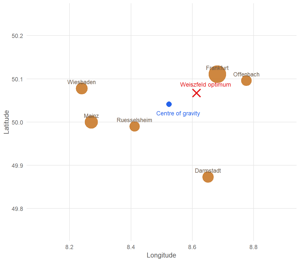
The centre of gravity is a centroid approximation of the Euclidean Steiner–Weber problem (here: longitude/latitude treated approximately as planar coordinates):

\[ x^{CoG} = \frac{\sum_{i=1}^{n} a_i u_i}{\sum_{i=1}^{n} a_i}, \qquad y^{CoG} = \frac{\sum_{i=1}^{n} a_i v_i}{\sum_{i=1}^{n} a_i}. \] For the SushiFresh example:

\[ (x^{CoG}, y^{CoG}) = (8.5241; 50.0410). \]

The centre of gravity is quick to compute, but only an approximation: in the example, the iterative Steiner–Weber location has a lower demand-weighted total haversine distance (1.4016^{4} vs. 1.409^{4} box-km).

Continuous Facility Location Planning

Steiner–Weber model with Manhattan distances

Steiner–Weber model with Manhattan distances

Determine coordinates $(x,y)$ in the sales area that minimise the weighted total transport distance to the customer locations.

\[ \min \; Z(x,y) = \sum_{i=1}^{n} a_i \left( |x-u_i| + |y-v_i| \right) = \sum_{i=1}^{n} a_i |x-u_i| + \sum_{i=1}^{n} a_i |y-v_i| \]

Algorithm for the optimal location

Determine the weighted median for each dimension — shown here for the $x$-coordinate (longitude):

Sort the stores by ascending $u_i$-coordinates.
Determine the cumulative demand $A_j = \sum_{i=1}^{j} a_i$.
Choose the first customer with $A_j \geq \frac{1}{2}\sum_{i=1}^{n} a_i$.
Its $u_i$-coordinate is the optimal $x$-coordinate.

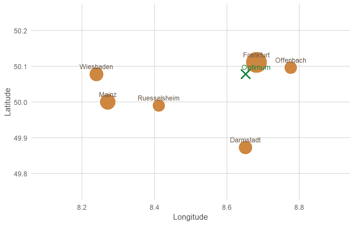
For the SushiFresh example: \[ (x^*, y^*) = (8.6512; 50.0782) \]

Strategic Design of Supply Chains

Multi-criteria facility location planning
Continuous facility location planning
Discrete facility location planning

Learning objectives

After this unit, you will be able to …

formulate discrete facility location and network design problems,
model transport, transshipment and location decisions in a network,
interpret key decision variables, objective functions and constraints,
evaluate the results of discrete network models for strategic location decisions.

Further reading

Transportation, transshipment and network models: (Günther and Tempelmeier 2012, chap. 4).
Discrete location models, algorithms and applications: Chapters 1–4 in (Daskin 2013).
Theory and applications of facility location: (Drezner and Hamacher 2002).

Planning Distribution Networks

Context

$\rightarrow$ Select specific locations in the network $\rightarrow$ usually a limited view of the SC

Case study – SushiFresh GmbH

Initial situation

Problem statement

SushiFresh GmbH supplies six supermarket stores in the Rhine-Main area daily with freshly produced sushi boxes. In Chapter 4, a qualitative pre-selection of locations using AHP was carried out (result: Mainz-Hechtsheim narrowly ahead), as well as a continuous location optimisation (centre of gravity/Weiszfeld). The question now is: does this result also hold up under a cost-based assessment?

Review of Chapter 4

AHP evaluation: Raunheim narrowly ahead
Centre of gravity / Weiszfeld: optimal point in the middle of the Rhine-Main area, near Raunheim
Open question: does a cost optimisation (fixed costs + transport) confirm this picture?

Case study – SushiFresh GmbH

Decision situation

Decision situation

SushiFresh must decide which of the three candidate locations will be developed for production and distribution, and which store should be supplied from which location. The company wants to make this decision so that the annual total costs of fixed costs and transport are minimised. The following information is known:

Candidate locations and annual fixed costs

ID	Location	Longitude	Latitude	Fixed costs/year (€1,000)
S1	Wiesbaden-Erbenheim	8.29990	50.06320	36
S2	Mainz-Hechtsheim	8.28310	49.96980	42
S3	Raunheim	8.46500	50.00000	52
S4	Höchst	8.54218	50.11146	48
S5	Isenburg	8.70720	50.05430	40

Transport distances in km

	C1	C2	C3	C4	C5	C6
S1	6.174	20.739	23.737	27.576	42.998	9.110
S2	4.603	25.745	29.584	44.289	36.928	39.002
S3	24.084	13.601	8.518	27.325	22.386	6.296
S4	30.588	33.354	44.696	16.751	34.263	37.121
S5	25.113	43.756	45.288	30.370	16.021	5.700

Stores and daily demand

ID	Store	Longitude	Latitude	Demand $\mu$ (boxes/day)
C1	Wiesbaden	8.2398	50.0782	120
C2	Mainz	8.2711	50.0000	150
C3	Frankfurt	8.6821	50.1109	280
C4	Rüsselsheim	8.4116	49.9904	90
C5	Darmstadt	8.6512	49.8728	110
C6	Offenbach	8.7761	50.0956	95

Warehouse Location Problem

Problem description

Problem statement

Consider a set of customer locations and a set of (potential) warehouse locations. Each customer location has a demand for goods (e.g. in units per month/year) that must be supplied by the warehouses. Transporting the goods incurs distance-dependent transport costs. Opening a warehouse incurs set-up costs.

The decision is at which locations warehouses should be set up and which customers they should supply.

Notation

Set of warehouses $i \in I$
Set of customer locations $j \in J$
Transport links $E \subseteq I \times J$
Opening costs at warehouse location $i$: $f_i$
Transport costs (e.g. in €/month) from location $i$ to customer $j$: $c_{ij}$
Demand of customer $j$: $a_j$

Warehouse Location Problem

Mathematical model

Mixed-integer linear programming model

Minimise the total costs of transport and opening locations

\[\min \rightarrow \sum_{i \in I} y_i \cdot f_i + \sum_{(i,j) \in E} x_{ij} \cdot c_{ij}\]

Constraints \[ \begin{align} \sum_{(i,j) \in E} x_{ij} &= a_j & \forall j \in J &\quad\rightarrow \text{satisfy demand} \\ x_{ij} &\leq y_i \cdot a_j & \forall (i,j) \in E &\quad\rightarrow \text{transport only from opened locations} \\ x_{ij} &\geq 0 & \forall (i,j) \in E &\quad\rightarrow \text{transport quantities non-negative} \\ y_i &\in \{0,1\} & \forall i \in I &\quad\rightarrow \text{location is opened or not} \end{align} \]

Warehouse Location Problem

Case example

Locations – fixed costs $f_i$ (€/year)

Location i	f_i (€)
S1	36,000
S2	42,000
S3	52,000
S4	48,000
S5	40,000

Stores – demand $a_j$ (boxes/year)

Store j	a_j
C1	120,000
C2	150,000
C3	280,000
C4	90,000
C5	110,000
C6	95,000

Transport costs $c_{ij}$ (€/box)

	C1	C2	C3	C4	C5	C6
S1	0.123	0.415	0.475	0.552	0.860	0.182
S2	0.092	0.515	0.592	0.886	0.739	0.780
S3	0.482	0.272	0.170	0.546	0.448	0.126
S4	0.612	0.667	0.894	0.335	0.685	0.742
S5	0.502	0.875	0.906	0.607	0.320	0.114

Warehouse Location Problem

Implementation with R/OMPR

library(ompr)
library(ompr.roi)
library(ROI.plugin.glpk)

# Problem data
n_I <- 5; n_J <- 6
f   <- c(36000, 42000, 52000, 48000, 40000)
a   <- c(120000, 150000, 280000, 90000, 110000, 95000)
c_ij <- matrix(
  c(
    0.12348,    0.41478,    0.47474,    0.55152,    0.85996,    0.18220,
    0.09206,    0.51490,    0.59168,    0.88578,    0.73856,    0.78004,
    0.48168,    0.27202,    0.17036,    0.54650,    0.44772,    0.12592,
    0.61176,    0.66708,    0.89392,    0.33502,    0.68526,    0.74242,
    0.50226,    0.87512,    0.90576,    0.60740,    0.32042,    0.11400),
  nrow = n_I, byrow = TRUE)

# MILP model
model <- MIPModel() |>
  # Variables
  add_variable(y[i], i = 1:n_I, type = "binary") |>
  add_variable(x[i,j], i = 1:n_I, j = 1:n_J,
               type = "continuous", lb = 0) |>
  # Objective function
  set_objective(
    sum_expr(f[i] * y[i], i = 1:n_I) +
    sum_expr(c_ij[i,j] * x[i,j],
             i = 1:n_I, j = 1:n_J),
    sense = "min") |>
  # C1: satisfy demand completely
  add_constraint(
    sum_expr(x[i,j], i = 1:n_I) == a[j],
    j = 1:n_J) |>
  # C2: transport only from opened warehouses
  add_constraint(
    x[i,j] <= y[i] * a[j],
    i = 1:n_I, j = 1:n_J)

result <- solve_model(model,
           with_ROI(solver = "glpk", verbose = FALSE))

OMPR – workflow

MIPModel() → empty model
add_variable() → decision variables
set_objective() → objective function
add_constraint() → constraints
solve_model() → call solver
get_solution() → extract solution

# Extract optimal solution
y_sol <- get_solution(result, y[i])
x_sol <- get_solution(result, x[i,j])

# Opened warehouses
offene_lager <- y_sol$i[y_sol$value > 0.5]

# Optimal objective value
obj_val <- objective_value(result)

Warehouse Location Problem

Case example – optimal solution

Location $i$	Store $j$	Quantity $x_{ij}$ (boxes)	Transport costs (€)
S1	C1	120,000	14,817.6
S3	C2	150,000	40,803.0
S3	C3	280,000	47,700.8
S3	C4	90,000	49,185.0
S3	C5	110,000	49,249.2
S3	C6	95,000	11,962.4

Cost type	€/year
Fixed costs	88,000
Transport costs	213,718
Total costs Z*	301,718

Warehouse Location Problem

Heuristic solution methods – basic ideas

Why heuristics?

The WLP is NP-hard: exact solvers (MILP) do find optimal solutions, but the computing time grows exponentially with $|I|$ and $|J|$. For large real-world instances, constructive heuristics are often the only practicable approach.

Basic idea

start with a feasible solution and try to improve it step by step
Each step: greedy – choose the change with the largest cost reduction
Stop when no further improvement is possible
Customers are always assigned to the cheapest open warehouse

Two classic approaches

Method	Starting point	Direction
Add heuristic	No warehouses open	Add step by step
Drop heuristic	All warehouses open	Close step by step

Basic ideas of add/drop – graphical

Warehouse Location Problem

Add heuristic

Idea: Start with no open warehouse. In each step, add the warehouse $i^*$ that reduces the total costs the most.

Algorithm

Initialisation: $S \leftarrow \emptyset$

Repeat:

For each warehouse not yet opened $i \notin S$, calculate the cost contribution: \[\Delta_i = Z(S) - Z(S \cup \{i\})\]
Choose $i^* = \arg\max_{i \notin S} \Delta_i$
If $\Delta_{i^*} > 0$: open $i^*$, set $S \leftarrow S \cup \{i^*\}$
Otherwise: stop

Assignment rule: Each customer $j$ is assigned to the cheapest open warehouse: $\sigma(j) = \arg\min_{i \in S} c_{ij}$

Cost calculation

\[Z(S) = \underbrace{\sum_{i \in S} f_i}_{\text{Opening}} + \underbrace{\sum_{j \in J} \min_{i \in S} c_{ij} \cdot a_j}_{\text{Transport}}\]

Properties:
- Greedy, not guaranteed to be optimal
- Transport costs decrease from step to step
- A new warehouse is opened if opening costs < transport cost savings

Stopping condition

The heuristic stops as soon as no further warehouse reduces the total costs.

Warehouse Location Problem

Drop heuristic

Idea: Start with all warehouses open. In each step, close the warehouse $i^*$ whose closure reduces the total costs the most.

Algorithm

Initialisation: $S \leftarrow I$

Repeat:

For each warehouse still open $i \in S$, calculate the cost contribution: \[\Delta_i = Z(S) - Z(S \setminus \{i\})\]
Choose $i^* = \arg\max_{i \in S} \Delta_i$
If $\Delta_{i^*} > 0$: close $i^*$, set $S \leftarrow S \setminus \{i^*\}$
Otherwise: stop

Assignment rule: $\sigma(j) = \arg\min_{i \in S} c_{ij}$

Comparison with add heuristic

Feature	Add	Drop
Start	$S = \emptyset$	$S = I$
Direction	constructive	destructive
Starting costs	$\infty$ (no warehouse)	$\sum_i f_i + \ldots$
Running time	$\mathcal{O}(\|I\|^2 \cdot \|J\|)$	$\mathcal{O}(\|I\|^2 \cdot \|J\|)$
Tendency	few warehouses	more warehouses

Important

Neither heuristic is guaranteed to be optimal. They deliver feasible solutions; the solution quality depends heavily on the cost structure of the instance.

Warehouse Location Problem

Add heuristic – case example

Step	Action	Open locations	Fixed costs (€)	Transport (€)	Total (€)
1	+S3	{S3}	52,000	256,702	308,702
2	+S1	{S1, S3}	88,000	213,718	301,718

Store assignment per step:

Step	C1	C2	C3	C4	C5	C6
1	S3	S3	S3	S3	S3	S3
2	S1	S3	S3	S3	S3	S3

Add heuristic result: location $\{S1, S3\}$ opened, $Z_\text{Add} = 301 718$ €/year

Warehouse Location Problem

Drop heuristic – case example

Step	Action	Open locations	Fixed costs (€)	Transport (€)	Total (€)
0	Start	{S1, S2, S3, S4, S5}	218,000	175,779.0	393,779.0
1	-S2	{S1, S3, S4, S5}	176,000	179,549.4	355,549.4
2	-S4	{S1, S3, S5}	128,000	198,582.6	326,582.6
3	-S5	{S1, S3}	88,000	213,718.0	301,718.0

Store assignment per step:

Step	C1	C2	C3	C4	C5	C6
0	S2	S3	S3	S4	S5	S5
1	S1	S3	S3	S4	S5	S5
2	S1	S3	S3	S3	S5	S5
3	S1	S3	S3	S3	S3	S3

Drop heuristic result: location $\{S1, S3\}$ opened, $Z_\text{Drop} = 301 718$ €/year — identical to the result of the add heuristic!

Warehouse Location Problem

Comparison of solutions

Metric	Optimum (MILP)	Add heuristic	Drop heuristic
Opened locations	S1, S3	S1, S3	S1, S3
Number of locations	2	2	2
Fixed costs (€)	36000	88000	88000
Transport costs (€)	265718	213718	213718
Total costs Z (€)	301718	301718	301718
Gap to optimum (%)	–	0%	0%

In this case example, the add heuristic and the drop heuristic independently find the same, provably optimal solution ($Z = 301 718$ €/year, only location S1 = Wiesbaden-Erbenheim). This is by no means a given, but here it shows the clear cost advantage of this location.

Cost comparison

Qualitative vs. Quantitative Location Assessment

Discussion

A contradiction with Chapter 4?

The AHP analysis in Chapter 4 narrowly favoured Mainz-Hechtsheim. The quantitative WLP analysis in this chapter favours Wiesbaden-Erbenheim and Raunheim. How do these fit together?

Location (single site)	Fixed costs (€)	Transport (€/year)	Total (€/year)
Raunheim	260,000	256,702.0	516,702.0
Wiesbaden-Erbenheim	180,000	371,503.2	551,503.2

Raunheim and Wiesbaden-Erbenheim have lower transport costs; the savings compensate for the higher fixed costs.

Conclusion

AHP (Chapter 4): good for an initial pre-selection based on soft criteria that are hard to quantify
WLP (Chapter 5): delivers the robust cost-based decision once hard figures are available
The two methods complement each other – neither replaces the other

SushiFresh decision

Consolidation of the production site at Wiesbaden-Erbenheim. This decision is revisited in Chapter 6 (risk pooling) and Chapter 8 (bullwhip effect).

Uncertainty and Risk Management in Supply Chains

Uncertainty in Supply Chains

Pooling
Newsvendor model
Bullwhip effect

Learning objectives

After this unit you will be able to …

explain sources and effects of uncertainty in supply chains,
distinguish between demand uncertainty, implied uncertainty and responsiveness,
analyse the effect of risk pooling on demand variance and safety stocks,
compare and assess centralised and decentralised inventory structures under uncertainty.

Further reading

Pooling, demand variability and inventory decisions: (Cachon and Terwiesch 2024, chaps. 10–13).
Safety stocks, service levels and inventory management: (Silver et al. 2017, chaps. 6–8).

Case study: SushiFresh GmbH

Six stores, one new central plant

Initial situation

SushiFresh GmbH is a fictitious regional producer of fresh sushi boxes in the Rhine-Main area, supplying six stores daily. In Chapter 5, the decision was made to consolidate production at one central site in Wiesbaden-Erbenheim. This chapter asks: how much safety stock is needed — decentralised vs. centralised?

Store	μ (boxes/day)	σ
Wiesbaden	120	25
Mainz	150	30
Frankfurt	280	55
Rüsselsheim	90	20
Darmstadt	110	24
Offenbach	95	22

Total demand: 845 boxes/day. Frankfurt (bold) is the largest and most volatile store.

The nature of uncertainty

Implied uncertainty in supply chains (Chopra and Meindl 2025)

Implied uncertainty denotes the uncertainty a supply chain must cope with — determined by the combination of demand uncertainty and the market’s service requirements (Chopra and Meindl 2025, Ch. 2).

Two sources of implied uncertainty

Dimension	Low	High
Demand uncertainty	Salt, electricity	Fashion, electronics
Supply variability	Concrete, coal	Semiconductors, fishing

$\rightarrow$ High implied uncertainty requires responsive supply chains with buffer capacity.

The basic dilemma

Demand is variable and hard to predict
Capacities (plants, warehouses, staff) are fixed in advance
$\rightarrow$ A mismatch between supply and demand is structurally unavoidable

The nature of uncertainty

Mismatch: fluctuating demand vs. fixed capacity

Capacities (machines, staff, storage space) are determined ex ante. Demand materialises ex post. The result: a systematic mismatch in both directions.

Consequences of the mismatch

Scenario	Phenomenon	Consequence
$d > C$	Overload	Lost sales, loss of revenue
$d < C$	Underutilisation	Idle costs
$d \approx C$	Equilibrium	with a perfect forecast

Practical examples

Automotive industry: plants produce only certain models for several years $\rightarrow$ utilisation depends on demand
Retail: seasonal goods (Christmas items) are ordered too early, leftovers are sold off cheaply
Hospital: operating theatre capacities are fixed daily, emergency volume is highly variable

Dealing with uncertainty

Capacity pooling

Initial situation (structure following Cachon & Terwiesch, Ch. 17)

In its start-up phase, SushiFresh initially operated only 2 pilot kitchens for 2 pilot sites (today’s Wiesbaden and Mainz stores). Each kitchen is assigned exclusively to its own site – no flexibility. Capacity per kitchen is 90 boxes/day. Demand is uncertain and is observed after capacities have been fixed.

Consequences of inflexibility

If demand exceeds capacity $\rightarrow$ shortage (lost sales)
If demand falls below capacity $\rightarrow$ idle capacity
Both effects reduce system performance

Capacity pooling

Original configuration – each kitchen supplies only its assigned store

Monthly demand and production, pilot phase ($C^{Wi} = C^{Ma} = 90$)

Month	d_t^Wi	d_t^Ma	x_t^Wi	x_t^Ma
1	78	102.0	78.00	90.00
2	79	92.0	79.00	90.00
3	92	93.0	90.00	90.00
4	76	87.0	76.00	87.00
5	95	80.0	90.00	80.00
6	104	97.0	90.00	90.00
7	87	90.0	87.00	90.00
8	92	76.0	90.00	76.00
9	91	89.0	90.00	89.00
10	85	86.0	85.00	86.00
11	96	89.0	90.00	89.00
12	93	93.0	90.00	90.00
⌀	89	89.5	86.25	87.25

System Evaluation

Expected demand: $E(d^{Wi})=$ 89; $E(d^{Ma})=$ 89.5
Expected production: $E(x^{Wi})=$ 86.2; $E(x^{Ma})=$ 87.2
Site utilisation: $\frac{E(x^{Wi})}{C^{Wi}}=$ 95.8%; $\frac{E(x^{Ma})}{C^2}=$ 96.9%
Expected fill rate: $\frac{E(x^{Wi})}{E(d^{Wi})}=$ 97.2%; $\frac{E(x^{Ma})}{E(d^{Ma})}=$ 97.7%

Problem

Utilisation and fill rate are high, yet there are lost sales and underutilisation $\rightarrow$ Can helping each other out (capacity pooling) improve these KPIs?

Capacity pooling

One-sided pooling – the Wiesbaden kitchen can supply both sites

Month	d_t^Wi	d_t^Ma	x_t^Wi,Wi	x_t^Wi,Ma	x_t^2B
1	78	102	78	12	90
2	79	92	79	2	90
3	92	93	90	0	90
4	76	87	76	0	87
5	95	80	90	0	80
6	104	97	90	0	90
7	87	90	87	0	90
8	92	76	90	0	76
9	91	89	90	0	89
10	85	86	85	0	86
11	96	89	90	0	89
12	93	93	90	0	90

Pooling rule (if $d_t^{Ma} > C^{Ma}$ and $d_t^{Wi} < C^{Wi}$):

\[x_t^1 = d_t^{Wi} + \min(C^{Wi} - d_t^{Wi};\; d_t^{Ma} - C^{Ma})\] \[x_t^{Ma,Ma} = C^{Ma}\]

System Evaluation (Pooling)

Production plant 1: $E(x^{Wi})=$ 87.4
Supply to market B: $E(x^{Wi,Ma}+x^{Ma,Ma})=$ 88.4
Utilisation plant 1: $\frac{E(x^{Wi})}{C^{Wi}}=$ 97.1%
Fill rate market B: $\frac{E(x^{Wi,Ma}+x^{Ma,Ma})}{E(d^{Ma})}=$ 98.8%

Capacity pooling

Two-sided pooling – both kitchens can supply both sites

Month	d_t^Wi	d_t^Ma	x_t^Wi,Wi	x_t^Wi,Ma	x_t^Ma,Ma	x_t^Ma,Wi
1	78	102	78	12	90	0
2	79	92	79	2	90	0
3	92	93	90	0	90	0
4	76	87	76	0	87	0
5	95	80	90	0	80	5
6	104	97	90	0	90	0
7	87	90	87	0	90	0
8	92	76	90	0	76	2
9	91	89	90	0	89	1
10	85	86	85	0	86	0
11	96	89	90	0	89	1
12	93	93	90	0	90	0

System Evaluation

Production Wiesbaden: $E(x^{Wi})=$ 87.4
Production Mainz: $E(x^{Ma})=$ 88
Supply to Wiesbaden: $E(x^{Wi, Wi}+x^{Ma, Wi})=$ 87
Supply to Mainz: $E(x^{Wi,Ma}+x^{Ma, Ma})=$ 88.4
Utilisation Wiesbaden: $\frac{E(x^{Wi})}{C^{Wi}}=$ 97.1%
Utilisation plant 2: $\frac{E(x^{Ma})}{C^{Ma}}=$ 97.8%
Fill rate Wiesbaden: $\frac{E(x^{Wi,Wi}+x^{Ma,Wi})}{E(d^{Wi})}=$ 97.8%
Fill rate Mainz: $\frac{E(x^{Ma,Ma}+x^{Wi,Ma})}{E(d^{Ma})}=$ 98.8%

The supply system behaves as if the separation between markets/products and plants were removed $\rightarrow$ total capacity and total demand are decisive

Capacity pooling

KPI comparison

KPI	Decentralised	One-sided pooling	Two-sided pooling
Ø Production Wiesbaden (units)	86.2	87.4	87.4
Ø Production Mainz (units)	87.2	87.2	88.0
Ø Sales Wiesbaden (units)	86.2	86.2	87.0
Ø Sales Mainz (units)	87.2	88.4	88.4
Lost sales Wiesbaden (units)	33.0	33.0	24.0
Lost sales Mainz (units)	27.0	13.0	13.0
Utilisation Wiesbaden (%)	95.8	95.8	96.7
Utilisation Mainz (%)	96.9	98.2	98.2
Sales ratio Wiesbaden (%)	96.9	96.9	97.8
Sales ratio Mainz (%)	97.5	98.8	98.8

Benefits of capacity pooling

Capacity pooling improves all service KPIs at once: more sales, higher utilisation, less idle capacity – without additional production capacity.

Costs of capacity pooling

However, capacity pooling requires additional logistics capacity and, above all, technological flexibility

Capacity pooling

Chaining

Chaining

Capacity pooling enables capacities to be shared across different markets. However, it requires technological and logistical flexibility. The more markets and products that need to be served, the more complex and costly capacity pooling becomes. So the question is: how can capacity pooling be organised for multiple products and markets?

Full chaining

Links: $n \cdot n = 16$

Technologies per plant: $n=4$

Markets per plant: $n=4$

Short chaining

Links: $2 \cdot n = 8$

Technologies per plant: $n=2$

Markets per plant: $n=2$

Long chaining

Links: $2 \cdot n = 8$

Technologies per plant: $n=2$

Markets per plant: $n=4$

Dealing with uncertainty

Pooling over time - safety stocks

Definition of safety stock (recap)

Safety stocks buffer demand fluctuations over time. Let $S$ be the initial inventory at the start of the risk period and $\mu$ the expected demand in the risk period; then the safety stock $sb$ is: $sb = S - \mu$

Example: the Wiesbaden-Erbenheim central plant periodically orders crates of fresh salmon fillet from the fish wholesaler.

Setting safety stocks

by cost: safety stocks incur inventory holding costs and avoid shortage costs $\rightarrow$ cost trade-off
Service readiness: protection against the risk of being unable to deliver during the risk period ($\alpha$ service level)
Fill rate: share of demand to be met within the risk period in the long run ($\beta$ service level)

Safety stocks

$\alpha$ service level and empirical distribution function

Assume that a stockout risk of 5% is acceptable, so the $\alpha$ service level is 95%. Question: which (minimum) initial inventory ensures this service level? Answer: Formally, $P(d \leq S) \geq \alpha$ must hold. For an empirical demand distribution $F(d)$ we therefore need $\hat{F}(S) \geq \alpha$ or $S \geq \hat{F}^{-1}(\alpha)$. So we are looking for an (empirical) quantile.

μ = 89 | n = 12
Rank	d_t	Count	F̂(d)
1	76	1	8.3%
2	78	1	16.7%
3	79	1	25%
4	85	1	33.3%
5	87	1	41.7%
6	91	1	50%
7	92	2	66.7%
8	93	1	75%
9	95	1	83.3%
10	96	1	91.7%
11	104	1	100%

Safety stocks $sb=S-\mu$: $sb_{75\%}=4$, $sb_{90\%}=7$, $sb_{95\%}=15$

Inventory pooling

Safety stocks with decentralised and centralised inventory holding

Decentralised network

Centralised network (pooling)

Safety stock savings: $sb_{decentral}=sb_{A}+sb_{B}=27.5$ vs. $sb_{0}=22.5$ $\rightarrow$ 5 units or 18%

Inventory pooling

Safety stocks with a known demand distribution

Demand distribution

It is often assumed that demand for goods in a given time span is a random variable whose distribution parameters (such as mean and variance) are known or can be estimated. Real data often deviate from this — simulated using the example of Frankfurt/Offenbach with occasional, shared holiday peaks.

Data basis: simulated daily demand over 250 days (set.seed(616), see R code for details)

ECDF (solid) = empirical distribution
Normal distribution (dotted) = parametric model

Store	μ̂	σ̂	KS p-value	emp. SS (α=95%)	param. SS
Frankfurt	294	65	0.000	366	400
Offenbach	95	23	0.001	120	132

The shared holiday peaks produce a right-skewed distribution in both stores that deviates clearly from the normal distribution (KS test: p < 0.01 for both) — accordingly, the empirical safety stock turns out lower than the parametric one.

Inventory pooling

Normally distributed demand – safety stock for two sites

Let $D_1 \sim \mathcal{N}(\mu_1, \sigma_1^2)$ and $D_2 \sim \mathcal{N}(\mu_2, \sigma_2^2)$ be the normally distributed demands at two sites with correlation $\rho = \text{Cor}(D_1, D_2)$.

The safety stock at site $i$ for an $\alpha$ service level is: $sb_i = z_\alpha \cdot \sigma_i$, so that in total: $sb_{dec} = z_\alpha \cdot (\sigma_1 + \sigma_2)$

Central warehouse: distribution of total demand

The aggregated demand $D_0 = D_1 + D_2$ is also normally distributed:

\[D_0 \sim \mathcal{N}\!\left(\mu_1 + \mu_2,\; \sigma_1^2 + \sigma_2^2 + 2\rho\,\sigma_1\sigma_2\right)\]

Hence the central safety stock is:

\[sb_{cen} = z_\alpha \cdot \sqrt{\sigma_1^2 + \sigma_2^2 + 2\rho\,\sigma_1\sigma_2}\]

Comparison: decentralised vs. centralised

Configuration	Safety stock
Decentralised (2 warehouses)	$z_\alpha \cdot (\sigma_1 + \sigma_2)$
Centralised ($\rho = -1$)	$z_\alpha \cdot \\|\sigma_1 - \sigma_2\\|$
Centralised ($\rho = 0$)	$z_\alpha \cdot \sqrt{\sigma_1^2 + \sigma_2^2}$
Centralised ($\rho = +1$)	$z_\alpha \cdot (\sigma_1 + \sigma_2)$

$\rightarrow$ $\|\sigma_1 - \sigma_2\| \leq \sqrt{\sigma_1^2 + \sigma_2^2} \leq \sigma_1 + \sigma_2$ $\rightarrow$ Pooling pays off as long as $\rho < 1$

The smaller the correlation $\rho$, the greater the savings potential from central pooling. (risk-balancing effect)

Key result

Safety stock for all six SushiFresh stores ($\alpha = 95\%$)

Verified with qnorm()

$z_{0.95} =$ 1.645
Decentralised: $sb_{dec}=z_\alpha\sum\sigma_i=$ 289.5 boxes
Centralised (pooled, independent): $sb_{cen}=z_\alpha\sqrt{\sum\sigma_i^2}=$ 127.5 boxes
Savings from consolidation: 56%

Cross-check pooling_safety_stock(): for 6 identical stores with $\bar\sigma=$ 29.3 the savings would be 59% — more than the actual 56%. The dominant, volatile Frankfurt site ($\sigma=55$) reduces the relative pooling advantage compared with the idealised case of equally sized sites.

56.0% less safety stock through centralisation at Wiesbaden-Erbenheim — at an identical service level.

Inventory pooling

Empirical illustration

Negative correlation $\rho = -0.8$

No correlation $\rho = 0$

Positive correlation $\rho = +0.8$

With negative correlation, the fluctuations in $D_0$ dampen each other — total demand is more stable than the individual demands. With positive correlation, they reinforce each other.

Inventory pooling

Safety stock as a function of the correlation $\rho$

Three scenarios (Frankfurt $\sigma_1=25$, Offenbach $\sigma_2=30$, $\alpha = 95\%$)

$\rho$	$sb_{cen}$	Savings
$-0.8$	29.7	67.2%
$\;\;\;0$	64.2	29%
$+0.8$	85.9	5.1%
$(+1)$	90.5	0%

$sb_{dec} = z_\alpha \cdot (\sigma_1 + \sigma_2) =$ 90.5

Centralisation gain if $\sigma_1 \neq \sigma_2$

\[1-\frac{sb_{cen}}{sb_{dec}} = 1-\frac{\sqrt{\sigma_1^2 + \sigma_2^2 + 2\rho\,\sigma_1\sigma_2}}{\sigma_1 + \sigma_2}\]

Centralisation gain if $\sigma_1 = \sigma_2$

\[1-\frac{sb_{cen}}{sb_{dec}} = 1-\sqrt{\frac{1+\rho}{2}}\]

Inventory pooling

Simulated daily demand: Frankfurt & Offenbach

KPI	Frankfurt	Offenbach	Total / pool
μ̂	294.1	94.9	389
σ̂	64.7	22.8	79.6
SS decentralised (emp.)	71.5	25.1	96.6
SS centralised (emp.)	—	—	80.5
Savings (emp.)	—	—	16.7%
SS decentralised (norm.)	106.4	37.5	143.9
SS centralised (norm.)	—	—	130.8
Savings (norm.)	—	—	9.1%

Correlation $\hat{\rho} =$ 0.55 $\rightarrow$ pooling savings, empirical: 16.7%, parametric: 9.1%

Aside: normal distribution

Probability density function & cumulative distribution function

Formal definition

The density function $f(x)$ gives the relative frequency with which a value $x$ occurs, and the cumulative distribution function $F(x)$ is the cumulative probability:

\[f(x) = \frac{1}{\sigma\sqrt{2\pi}}\,\exp\!\left(-\frac{(x-\mu)^2}{2\sigma^2}\right) \qquad F(x) = P(X \leq x) = \int_{-\infty}^{x} f(t)\,dt\]

Symmetry property and 68–95–99.7 rule:

\[F(-z) = 1 - F(z)\]

Range of values	Probability
$\mu \pm 1\sigma$	≈ 68.3%
$\mu \pm 2\sigma$	≈ 95.4%
$\mu \pm 3\sigma$	≈ 99.7%

Aside: standard normal distribution

z-transformation & standardisation

The z-transformation converts any normal distribution $X \sim \mathcal{N}(\mu, \sigma^2)$ into the standard normal distribution $Z \sim \mathcal{N}(0, 1)$:

\[Z = \frac{X - \mu}{\sigma} \quad \Rightarrow P(X \leq x) = P\!\left(Z \leq \frac{x-\mu}{\sigma}\right) = \Phi(z)\] $\rightarrow$ all $\mathcal{N}(\mu, \sigma^2)$ can be reduced to one table — the standard normal distribution table $\Phi(z)$

Important quantiles of $\mathcal{N}(0,1)$:

Service level $\alpha$	$z_\alpha = \Phi^{-1}(\alpha)$
90.0%	1.282
95.0%	1.645
97.5%	1.960
99.0%	2.326
99.9%	3.090

Aside: quantile/distribution table

Reading $\Phi(z)$ and its inverse $z_\alpha = \Phi^{-1}(\alpha)$

Φ(z) — standard normal distribution (z ≥ 0)
	+0.00	+0.01	+0.02	+0.03	+0.04	+0.05	+0.06	+0.07	+0.08	+0.09
0.0	0.5000	0.5040	0.5080	0.5120	0.5160	0.5199	0.5239	0.5279	0.5319	0.5359
0.1	0.5398	0.5438	0.5478	0.5517	0.5557	0.5596	0.5636	0.5675	0.5714	0.5753
0.2	0.5793	0.5832	0.5871	0.5910	0.5948	0.5987	0.6026	0.6064	0.6103	0.6141
0.3	0.6179	0.6217	0.6255	0.6293	0.6331	0.6368	0.6406	0.6443	0.6480	0.6517
0.4	0.6554	0.6591	0.6628	0.6664	0.6700	0.6736	0.6772	0.6808	0.6844	0.6879
0.5	0.6915	0.6950	0.6985	0.7019	0.7054	0.7088	0.7123	0.7157	0.7190	0.7224
0.6	0.7257	0.7291	0.7324	0.7357	0.7389	0.7422	0.7454	0.7486	0.7517	0.7549
0.7	0.7580	0.7611	0.7642	0.7673	0.7704	0.7734	0.7764	0.7794	0.7823	0.7852
0.8	0.7881	0.7910	0.7939	0.7967	0.7995	0.8023	0.8051	0.8078	0.8106	0.8133
0.9	0.8159	0.8186	0.8212	0.8238	0.8264	0.8289	0.8315	0.8340	0.8365	0.8389
1.0	0.8413	0.8438	0.8461	0.8485	0.8508	0.8531	0.8554	0.8577	0.8599	0.8621
1.1	0.8643	0.8665	0.8686	0.8708	0.8729	0.8749	0.8770	0.8790	0.8810	0.8830
1.2	0.8849	0.8869	0.8888	0.8907	0.8925	0.8944	0.8962	0.8980	0.8997	0.9015
1.3	0.9032	0.9049	0.9066	0.9082	0.9099	0.9115	0.9131	0.9147	0.9162	0.9177
1.4	0.9192	0.9207	0.9222	0.9236	0.9251	0.9265	0.9279	0.9292	0.9306	0.9319
1.5	0.9332	0.9345	0.9357	0.9370	0.9382	0.9394	0.9406	0.9418	0.9429	0.9441
1.6	0.9452	0.9463	0.9474	0.9484	0.9495	0.9505	0.9515	0.9525	0.9535	0.9545
1.7	0.9554	0.9564	0.9573	0.9582	0.9591	0.9599	0.9608	0.9616	0.9625	0.9633
1.8	0.9641	0.9649	0.9656	0.9664	0.9671	0.9678	0.9686	0.9693	0.9699	0.9706
1.9	0.9713	0.9719	0.9726	0.9732	0.9738	0.9744	0.9750	0.9756	0.9761	0.9767
2.0	0.9772	0.9778	0.9783	0.9788	0.9793	0.9798	0.9803	0.9808	0.9812	0.9817
2.1	0.9821	0.9826	0.9830	0.9834	0.9838	0.9842	0.9846	0.9850	0.9854	0.9857
2.2	0.9861	0.9864	0.9868	0.9871	0.9875	0.9878	0.9881	0.9884	0.9887	0.9890
2.3	0.9893	0.9896	0.9898	0.9901	0.9904	0.9906	0.9909	0.9911	0.9913	0.9916
2.4	0.9918	0.9920	0.9922	0.9925	0.9927	0.9929	0.9931	0.9932	0.9934	0.9936
2.5	0.9938	0.9940	0.9941	0.9943	0.9945	0.9946	0.9948	0.9949	0.9951	0.9952
2.6	0.9953	0.9955	0.9956	0.9957	0.9959	0.9960	0.9961	0.9962	0.9963	0.9964
2.7	0.9965	0.9966	0.9967	0.9968	0.9969	0.9970	0.9971	0.9972	0.9973	0.9974
2.8	0.9974	0.9975	0.9976	0.9977	0.9977	0.9978	0.9979	0.9979	0.9980	0.9981
2.9	0.9981	0.9982	0.9982	0.9983	0.9984	0.9984	0.9985	0.9985	0.9986	0.9986
3.0	0.9987	0.9987	0.9987	0.9988	0.9988	0.9989	0.9989	0.9989	0.9990	0.9990

Reading the table:
Wanted: $P(X \leq x)$ for $X \sim \mathcal{N}(\mu, \sigma^2)$

Compute $z = (x - \mu)/\sigma$
Row = first decimal place of $z$
Column = second decimal place of $z$
Table value = $\Phi(z)$

Inventory example:
$D \sim \mathcal{N}(500, 80^2)$, service level $\alpha = 95\%$

\[z_{0.95} = \Phi^{-1}(0.95) = 1.645\]

\[\Rightarrow\; \text{SS} = z_\alpha \cdot \sigma = 1.645 \cdot 80 \approx \mathbf{132\;\text{units}}\]

Uncertainty in Supply Chains

Risk pooling
Newsvendor model
Bullwhip effect

Learning objectives

After this unit you will be able to …

classify the newsvendor problem as a one-off ordering decision under uncertain demand,
determine overage and underage costs,
derive and interpret the critical fractile rule,
calculate an optimal order quantity for a given demand distribution,
explain the influence of key model parameters on the ordering decision.

Further reading

Introduction to the newsvendor model: (Thonemann 2023, chap. 5).
Single-period inventory models and critical fractile logic: (Cachon and Terwiesch 2024, chap. 13).
Newsvendor models in the context of inventory management: (Silver et al. 2017, chap. 9).

Case example

Sushi boxes in the supermarket

Every day, a supermarket sources freshly produced sushi boxes from SushiFresh GmbH, a regional sushi producer in the Rhine-Main region.

The boxes are prepared in the morning and delivered before the store opens.
Demand is uncertain until the evening. Replenishment during the day is not possible.
Unsold sushi boxes may not be sold at regular price on the following day.

Decision question: How many sushi boxes should the supplier prepare?

Case example

Cost and revenue structure

The following simplified values apply to a sushi box:

Quantity	Meaning	Value
Selling price $p$	Revenue per sushi box sold	€10
Production and delivery costs $c$	Cost per sushi box prepared	€5
Salvage value $v$	Revenue from evening discount or disposal	€2

In general, typically: $p > c > v$

$\rightarrow$ Contribution margin per sushi box sold: $c^u=p-c = 10-5=5$ €

$\rightarrow$ Salvage loss per unsold sushi box: $c^o=c-v=5-2=3$ €

Case example

Two possible situations from the supplier’s perspective

Too many boxes:

less demand $D$ than sushi boxes produced $q$ $\rightarrow$ excess stock $q-D$
quantity sold: $\min(D,q) = D$
contribution margin from sales: $D \cdot c^u$
additional salvage costs: $(q-D) \cdot c^o$

Total contribution margin: $P(D,q)= D \cdot c^u - (q - D) \cdot c^o$

Too few boxes:

more demand $D$ than sushi boxes produced $q$ $\rightarrow$ shortage $D-q$
quantity sold: $\min(D,q) = q$
total contribution margin: $q \cdot c^u$
opportunity costs from lost contribution margin: $(D-q) \cdot c^u$

Total contribution margin: $P(D,q) = q \cdot c^u$

Case example

Possible demand & production quantity

As a simplified miniature example (e.g. for a small store or a test sale), SushiFresh first estimates four possible demand scenarios from sales history, day of the week, weather forecast and current promotions:

Demand $D$	Probability $P(D=d)$	Cumulative probability $F(d)$
30 sushi boxes	0.20	0.20
40 sushi boxes	0.35	0.55
50 sushi boxes	0.30	0.85
60 sushi boxes	0.15	1.00

Which quantity should the supplier prepare in the morning: 30, 40, 50 or 60 sushi boxes?

Case example

Expected result

Set $q=40$ sushi boxes

Demand $D$	Prob. $P(D=d)$	Excess stock $q-D$	Shortage $q-D$	Contri-bution $P$
30 sushi boxes	0.20	10	0	€120
40 sushi boxes	0.35	0	0	€200
50 sushi boxes	0.30	0	10	€200
60 sushi boxes	0.15	0	20	€200

Expected total contribution margin: $\begin{align} E(P|q=40)= & 0.2 \cdot 120 + 0.35 \cdot 200 + \\ & 0.30 \cdot 200 + 0.15 \cdot 200= 184 \end{align}$

$E(P|q)$ for all $q$

$\rightarrow$ maximum expected contribution margin at $q=50$ with € 190 per day

Newsvendor model

Derivation of the objective function

Overage $q > D$

\[P(D,q) = D \cdot c^u - (q-D)^+\cdot c^o\]

\[\Downarrow\]

Underage $q < D$

\[P(D,q) = q \cdot c^u\]

\[\Downarrow\]

\[\begin{align} P(D,q) =& \min(D,q) \cdot c^u - (q-D)^+ \cdot c^o \\ = & (D-(D-q)^+) \cdot c^u - (q-D)^+ \cdot c^o \\ = & \underset{\text{contribution margin}}{D \cdot c^u} - \underset{\text{ shortage costs}}{(D-q)^+ \cdot c^u} - \underset{\text{excess stock costs}}{(q-D)^+ \cdot c^o} \end{align} \] where $(q-D)^+ = \max(0,q-D)$, $(D-q)^+ = \max(0,D-q)$ and $\min(D,q) = D - (D-q)^+$

Newsvendor model

Formal model

Problem description

Find the order quantity $q$ that maximises expected profit or minimises expected costs: \[ \underset{q}{\max} E(P(q)) = \mu \cdot c^u - E((D-q)^+) \cdot c^u - E((q-D)^+) \cdot c^o \; \Leftrightarrow \; \underset{q}{\min} E(C(q)) = E((D-q)^+) \cdot c^u + E((q-D)^+) \cdot c^o \] $\rightarrow$ minimise the weighted average of expected shortage $E((D-q)^+)$ and expected excess stock $E((q-D)^+)$

Discrete demand (cf. previous slide)

Continuous demand (Frankfurt store) $D \sim N(280,55^2)$

Newsvendor model

Formal solution

The optimal order quantity $q^*$ is where the slopes of the expected shortage costs $E((D-q)^+) \cdot c^u$ and the excess stock costs $E((q-D)^+)\cdot c^o$ are equal: \[ \left(1 - F(q^*)\right) \cdot c^u \overset{!}{=} F(q^*) \cdot c^o \quad \Longrightarrow \quad q^* = F^{-1} \left( \frac{c^u}{c^o + c^u} \right)\]

Discrete demand (distribution parameters cf. previous slide) with $c^u = 5$ and $c^o=3$

Continuous demand (Frankfurt store) $D \sim N(280,55^2)$ with $c^u = 5$ and $c^o=3$

Newsvendor model

Critical ratio

Critical ratio

The optimal order quantity is the demand quantile whose cumulative probability equals the ratio of shortage costs to total costs. The critical ratio thus determines the willingness to take risks

\[ CR = \frac{c^u}{c^o + c^u}\]

Case 1: $c^u < c^o$

Shortage costs are lower than excess stock costs
Excess stock should be avoided
$\rightarrow$ opt. order quantity $q^*$ smaller than the median of the demand distribution

Case 2: $c^u = c^o$

Shortage costs = excess stock costs
Shortages and excess stock equally important
$\rightarrow$ opt. order quantity $q^*$ equals the median of the demand distribution

Case 3: $c^u > c^o$

Shortage costs are higher than excess stock costs
Shortages should be avoided
$\rightarrow$ opt. order quantity $q^*$ larger than the median of the demand distribution

Newsvendor model

Optimal solution under normal distribution

Normally distributed demand

For normally distributed demand with $D \sim (\mu,\sigma^2)$, the optimal order quantity can be calculated by transforming to the standard normal distribution. For the optimal order quantity and costs: \[z^* = \Phi^{-1} \left( \frac{c^u}{c^o + c^u} \right) \qquad q^*=\mu + \sigma \cdot z^* \qquad E(C(q^*))=(c^u+c^o)\cdot \sigma \cdot \varphi\left( z^* \right) \]

Case example Frankfurt store with $N(280,55^2)$

Case 1: $c^u=1 < 5=c^o$

$q^* = 280 + 55 \cdot$ -0.97=226.8

Case 2: $c^u = 3 = c^o$

$q^* = 280 + 55 \cdot$ 0=280

Case 3: $c^u=5 > 1=c^o$

$q^* = 280 + 55 \cdot$ 0.97=333.2

Newsvendor model

Typical applications

Prerequisites

The newsvendor model is used particularly often when demand cannot be smoothed through inventory holding and shortage costs can be determined well

Typical areas of application include, e.g.

seasonal and promotional items
fresh products with a short shelf life
tickets for events or transport
…

Important

Beyond that, it is the basis for calculating cost-optimal safety stocks in inventory systems.

Uncertainty in supply chains

Risk pooling
Newsvendor model
Bullwhip effect

Learning objectives

After this unit you will be able to …

explain the bullwhip effect along a supply chain
assess the main causes and consequences of the bullwhip effect
determine the order-up-to level $S$ and safety stock $SB$
classify measures to reduce the bullwhip effect

Further reading

Fundamental causes of and countermeasures to the bullwhip effect: (Thonemann 2023, chap. 8, especially 8.2).
Empirical study of information transmission: (Bray and Mendelson 2012).
Measurement, aggregation and impact of bullwhip effects: (Yao et al. 2020).

Case example: sushi boxes

Continued

The SushiFresh supply chain

SushiFresh GmbH is a regional producer of fresh sushi boxes and supplies six supermarket stores in the Rhine-Main area. For production, SushiFresh depends on daily deliveries of fresh fish fillets supplied by the fish wholesaler Nord-Fisch KG. The sushi supply chain is therefore structured as follows:

\[ \text{Supermarket stores} \mathrel{ \mathop{\leftrightharpoons} \limits^{\text{Delivery}}_{\text{Order}} } \text{SushiFresh GmbH} \mathrel{ \mathop{\leftrightharpoons} \limits^{\text{Delivery}}_{\text{Order}} } \text{Nord-Fisch KG} \]

Supermarket stores

observe end-customer demand (e.g. Frankfurt store: $\mu=280$, $\sigma=55$)
order sushi boxes from SushiFresh daily

SushiFresh GmbH

receives orders from the stores (= demand)
orders fish for the sushi boxes from Nord-Fisch KG and keeps a stock of fish in reserve

Nord-Fisch KG

receives orders from SushiFresh GmbH (= demand)
sources raw fish, produces the fish fillets and stores them in order to deliver quickly

Important

SushiFresh and Nord-Fisch each hold a (safety) stock of fish fillets to avoid shortages $\rightarrow$ How high should it be?

Case example: SushiFresh GmbH

Situation of SushiFresh GmbH

Ordering process for fish fillets

SushiFresh GmbH decides daily on its production quantity of sushi boxes for the Frankfurt store (cf. newsvendor model slides). Based on sushi box demand, let $d_t$ be the demand for fish fillet units on day $t$ (Frankfurt store: $\mu=280$, $\sigma=55$). SushiFresh can order replenishment from Nord-Fisch KG every day. Let the order quantity on day $t$ be $q_t$. Ordered fish fillets are delivered $l=2$ days later. Let the physically available quantity of fish fillet units be $i_t$. If no fish fillets are in stock, the demand is backordered ($b_t$) and produced or delivered later.

Sushi box inventories

the physical inventory $i_t$ is calculated as $i_t = \max(0,i_{t-1} + q_{t-2} - d_t)$
the net inventory $n_t$ also accounts for shortages $n_t = i_{t-1} + q_{t-2} - d_t$
the inventory position $p_t$ also accounts for open orders $p_t = n_{t-1} + q_{t-1} (+q_t)$

Case example: SushiFresh GmbH

Inventory of SushiFresh GmbH (Frankfurt store)

Demand

Period	Demand
0	NA
1	234
2	256
3	344
4	410
5	278
6	322
7	212
8	256
9	278
10	234
11	256
12	278

Initial inventory $i_0 =$ 990 Order-up-to level $S =$ 990

Case example: SushiFresh GmbH

Setting the order-up-to level

Ordering process & order-up-to level $S$

Setting the order-up-to level $S$ determines the order quantity and the safety stock:

\[ q_t = S - p_t \qquad \qquad sb_t = S - \mu \cdot (l+1) \]

for a given $\alpha$ service level

Extending the single-period formula (cf. pooling lecture) to multiple periods:

\[ S = \mu \cdot (l+1) + \sqrt{l+1} \cdot \sigma \cdot z_{\alpha}\]

for a given shortage cost rate $c^u$ and inventory holding cost rate $c^o$

Applying the newsvendor formula:

\[ S = \mu \cdot (l+1) + \sqrt{l+1} \cdot \sigma \cdot z_{\frac{c^u}{c^u+c^o}}\]

Important

Important: the parameters $\mu$ and $\sigma$ are the expected daily demand (rate) (demand per period) and the expected deviation (standard deviation). Both parameters are estimated on the basis of empirical customer demand.

Case example: SushiFresh GmbH

Order decisions and their effects

Estimating the demand parameters $\mu$ and $\sigma$

The parameters of the demand distribution are determined using statistical estimation methods (estimators), such as the (moving) average and the empirical standard deviation:

$\hat{\mu} = \frac{1}{T} \sum_{\tau=t-T}^{t-1} d_\tau \qquad \qquad \hat{\sigma} = \sqrt{ \frac{1}{T-1} \sum_{\tau=t-T}^{t-1} (d_\tau - \hat{\mu})^2 } \rightarrow \;\text{forecast error}$

	1	2	3	4	5	6	7	8	9	10	11	12
Demand d[t]	234	256	344.0	410.0	278.0	322	212.0	256.0	278.0	234.0	256	278
Mean μ̂[t]	256	234	245.0	278.0	336.7	344	336.7	270.7	263.3	248.7	256	256
Standard deviation σ̂[t]	1	1	15.6	58.2	77.3	66	67.2	55.4	55.4	33.6	22	22
Order-up-to level S[t]	771	705	779.0	1000.0	1230.0	1220	1201.0	970.0	948.0	842.0	831	831
Order q[t]	15	190	418.0	631.0	508.0	312	193.0	25.0	256.0	128.0	245	278

Observation

The variability of demand $\sigma_d=$ 55.1 is considerably smaller than the standard deviation of the order quantities $\sigma_q=$ 183.1 $\rightarrow$ additional uncertainty is generated for Nord-Fisch KG

Bullwhip effect

Definition & illustration

Definition (Cachon and Terwiesch 2024)

The bullwhip effect is present in a supply chain if the variability of demand at one level of the supply chain is greater than the variability of demand at the next downstream level in the supply chain, where variability is measured with the coefficient of variation.

Typical patterns

Upstream effects

“Amplification” of order quantities
Inventory volatility increases
more frequent shortages

Bullwhip effect

Typical observations

usually $q_t \neq d_t$, since the order quantity contains several components \[ q_t=\text{expected demand}+\text{inventory correction}+\text{safety stock correction}.\]
suppliers cannot tell whether fluctuations in order quantities indicate long-term shifts (i.e. end-customer demand is rising) or short-term inventory corrections $\rightarrow$ estimating future demand is difficult $\rightarrow$ forecast errors increase $\rightarrow$ order quantities fluctuate more
hence the fluctuations of order quantities often increase with every stage of the value chain: $\operatorname{Var}(d_t)< \operatorname{Var}(q_t^{i})<\operatorname{Var}(q_t^{i+1})<\operatorname{Var}(q_t^{i+2})< ...$

Measuring the bullwhip effect

Measures of the bullwhip effect are the variance ratios $B=\frac{\operatorname{Var}(q_t)}{\operatorname{Var}(d_t)}>1$ and $B=\frac{\operatorname{Var}(q^{i}_t)}{\operatorname{Var}(q^{i-1}_t)}>1$

$\rightarrow$ the larger $B$, the stronger the bullwhip effect

Bullwhip effect

Empirical evidence (Bray and Mendelson 2012; Chen and Lee 2012; Yao et al. 2020)

$2/3$ of companies

In a sample of 4,689 listed US companies, around two thirds showed a positive amplification of procurement variability relative to sales variability.

$+15.8\%$ on average

The mean bullwhip amplification was $15.8\%$ of demand variability; the median was $6.7\%$.

Order of magnitude

On average, the quarterly standard deviation of upstream orders exceeded that of observed demand by around USD 20 million.

Real performance consequences (Yao et al. 2020)

A stronger bullwhip effect is associated with a higher inventory ratio and at the same time more stockouts $\rightarrow$ safety stocks are insufficient

Aggregation conceals the problem

Metrics aggregated across products, stores or time underestimate the bullwhip effect compared with measurement at SKU level.

Management message

It is not only end-customer demand that creates volatility:

\[ \text{demand signal} + \text{local ordering decisions} = \text{order variance} \]

Bullwhip effect

Causes of the bullwhip effect

Cause	Mechanism
Local forecasts	Orders are interpreted as actual demand
Forecast updating	Small changes in demand lead to adjustments of order-up-to levels
Long lead times	Decisions must take effect far into the future
Order batching	Infrequent large orders create artificial demand peaks
Price promotions	Forward buying distorts observed demand
Rationing	Actors strategically order more than their actual demand
Lack of transparency	End-customer demand is not visible to all stages
Local systems of objectives	Stages optimise individually rather than system-wide

Bullwhip effect

Typical consequences

Operational consequences

Fluctuating production schedules
Unstable capacity utilisation
Express shipments and special measures
High inventories and yet shortages
Lower delivery capability
Greater planning uncertainty

Economic consequences

Higher capital tie-up
Higher warehousing costs
Higher obsolescence risks
Higher set-up and production costs
Higher transport costs
Losses in revenue and contribution margin

Bullwhip effect

Countermeasures

Lever	Measure	Effect on inventories and variance
Information flow	Share point-of-sale data	$\sigma$ of forecast errors decreases
Planning	Joint forecasts and CPFR	Local forecast bias decreases
Ordering policy	Small, frequent orders	Order batching decreases
Lead time	Shorten information and delivery lead times	Risk period decreases
Prices	Stable prices instead of forward-buying incentives	Artificial demand peaks decrease
Allocation	Rationing based on historical quantities	Strategic over-ordering decreases
Control	Overall optimum instead of local targets	Order and inventory decisions are coordinated

Configuration	Safety stock
Decentralised (2 warehouses)	\(z_\alpha \cdot (\sigma_1 + \sigma_2)\)
Centralised (\(\rho = -1\))	\(z_\alpha \cdot \\|\sigma_1 - \sigma_2\\|\)
Centralised (\(\rho = 0\))	\(z_\alpha \cdot \sqrt{\sigma_1^2 + \sigma_2^2}\)
Centralised (\(\rho = +1\))	\(z_\alpha \cdot (\sigma_1 + \sigma_2)\)

Feature	Add	Drop
Start	\(S = \emptyset\)	\(S = I\)
Direction	constructive	destructive
Starting costs	\(\infty\) (no warehouse)	\(\sum_i f_i + \ldots\)
Running time	\(\mathcal{O}(\|I\|^2 \cdot \|J\|)\)	\(\mathcal{O}(\|I\|^2 \cdot \|J\|)\)
Tendency	few warehouses	more warehouses

Scenario	Phenomenon	Consequence
\(d > C\)	Overload	Lost sales, loss of revenue
\(d < C\)	Underutilisation	Idle costs
\(d \approx C\)	Equilibrium	with a perfect forecast

Month	d_t^Wi	d_t^Ma	x_t^Wi,Wi	x_t^Wi,Ma	x_t^2B
1	78	102	78	12	90
2	79	92	79	2	90
3	92	93	90	0	90
4	76	87	76	0	87
5	95	80	90	0	80
6	104	97	90	0	90
7	87	90	87	0	90
8	92	76	90	0	76
9	91	89	90	0	89
10	85	86	85	0	86
11	96	89	90	0	89
12	93	93	90	0	90

Month	d_t^Wi	d_t^Ma	x_t^Wi,Wi	x_t^Wi,Ma	x_t^Ma,Ma	x_t^Ma,Wi
1	78	102	78	12	90	0
2	79	92	79	2	90	0
3	92	93	90	0	90	0
4	76	87	76	0	87	0
5	95	80	90	0	80	5
6	104	97	90	0	90	0
7	87	90	87	0	90	0
8	92	76	90	0	76	2
9	91	89	90	0	89	1
10	85	86	85	0	86	0
11	96	89	90	0	89	1
12	93	93	90	0	90	0

\(\rho\)	\(sb_{cen}\)	Savings
\(-0.8\)	29.7	67.2%
\(\;\;\;0\)	64.2	29%
\(+0.8\)	85.9	5.1%
\((+1)\)	90.5	0%

Range of values	Probability
\(\mu \pm 1\sigma\)	≈ 68.3%
\(\mu \pm 2\sigma\)	≈ 95.4%
\(\mu \pm 3\sigma\)	≈ 99.7%

Quantity	Meaning	Value
Selling price \(p\)	Revenue per sushi box sold	€10
Production and delivery costs \(c\)	Cost per sushi box prepared	€5
Salvage value \(v\)	Revenue from evening discount or disposal	€2

Lever	Measure	Effect on inventories and variance
Information flow	Share point-of-sale data	\(\sigma\) of forecast errors decreases
Planning	Joint forecasts and CPFR	Local forecast bias decreases
Ordering policy	Small, frequent orders	Order batching decreases
Lead time	Shorten information and delivery lead times	Risk period decreases
Prices	Stable prices instead of forward-buying incentives	Artificial demand peaks decrease
Allocation	Rationing based on historical quantities	Strategic over-ordering decreases
Control	Overall optimum instead of local targets	Order and inventory decisions are coordinated

Month	d_t^Wi	d_t^Ma	x_t^Wi,Wi	x_t^Wi,Ma	x_t^2B
1	78	102	78	12	90
2	79	92	79	2	90
3	92	93	90	0	90
4	76	87	76	0	87
5	95	80	90	0	80
6	104	97	90	0	90
7	87	90	87	0	90
8	92	76	90	0	76
9	91	89	90	0	89
10	85	86	85	0	86
11	96	89	90	0	89
12	93	93	90	0	90

Month	d_t^Wi	d_t^Ma	x_t^Wi,Wi	x_t^Wi,Ma	x_t^Ma,Ma	x_t^Ma,Wi
1	78	102	78	12	90	0
2	79	92	79	2	90	0
3	92	93	90	0	90	0
4	76	87	76	0	87	0
5	95	80	90	0	80	5
6	104	97	90	0	90	0
7	87	90	87	0	90	0
8	92	76	90	0	76	2
9	91	89	90	0	89	1
10	85	86	85	0	86	0
11	96	89	90	0	89	1
12	93	93	90	0	90	0

Month	d_t^Wi	d_t^Ma	x_t^Wi,Wi	x_t^Wi,Ma	x_t^2B
1	78	102	78	12	90
2	79	92	79	2	90
3	92	93	90	0	90
4	76	87	76	0	87
5	95	80	90	0	80
6	104	97	90	0	90
7	87	90	87	0	90
8	92	76	90	0	76
9	91	89	90	0	89
10	85	86	85	0	86
11	96	89	90	0	89
12	93	93	90	0	90

Month	d_t^Wi	d_t^Ma	x_t^Wi,Wi	x_t^Wi,Ma	x_t^Ma,Ma	x_t^Ma,Wi
1	78	102	78	12	90	0
2	79	92	79	2	90	0
3	92	93	90	0	90	0
4	76	87	76	0	87	0
5	95	80	90	0	80	5
6	104	97	90	0	90	0
7	87	90	87	0	90	0
8	92	76	90	0	76	2
9	91	89	90	0	89	1
10	85	86	85	0	86	0
11	96	89	90	0	89	1
12	93	93	90	0	90	0